Other Applications
This chapter presents two shorter investigations which use Graph Diffusion Distance.
Shape Analysis for Discretized Meshes
In this section we demonstrate that graph diffusion distance captures structural properties of 3D point clouds. Ten 3D meshes (see Figure [fig:mesh_grid] for an illustration of the meshes used) were chosen to represent an array of objects with varying structural and topological properties. Not all of the mesh files chosen are simple manifolds: for example, the “y-tube" is an open-ended cylinder with a fin around its equator. Each mesh was used to produce multiple graphs, via the following procedure:
[sample_step_a] Subsampling the mesh to 1000 points;
Performing a clustering step on the new point cloud to identify 256 cluster centers;
Connecting each cluster center to its 16 nearest neighbors in the set of cluster centers.
Since each pass of this procedure (with different random seeds) varied in Step [sample_step_a], each pass produced a different graph. We generated 20 graphs for each mesh, and compared the graphs using GDD.
[fig:mesh_grid]
The results of this experiment can be seen in Figure [fig:gdd_of_meshes]. This Figure shows the three first principal components of the distance matrix of GDD on the dataset of graphs produced as described above. Each point represents one graph in the dataset, and is colored according to the mesh which was used to generate it. Most notably, all the clusters are tight and do not overlap. Close clusters represent structurally similar objects: for example, the cluster of graphs from the tube mesh is very close to the cluster derived from the tube with an equatorial fin. This synthetic dataset example demonstrates that graph diffusion distance is able to compare structural information about point clouds and meshes.
[fig:gdd_of_meshes]
Morphological Analysis of Cell Networks
In this section, we present an application of GDD to biological image analysis, and a generalization of GDD that makes it more suitable for machine learning tasks.
Biological Background
Species in the plant genus Arabidopsis are of high interest in plant morphology studies, since 1) its genome was fully sequenced in 1996, relatively early (Kaul et al. 2000), and 2) its structure makes it relatively easy to capture images of the area of active cell division: the shoot apical meristem (SAM). Recent work (Schaefer et al. 2017) has found that mutant Arabidopsis specimens with a decreased level of expression of genes trm6,trm7, and trm8 demonstrate more variance in the placement of new cell walls during cell division.
We prepare a dataset of Arabidopsis images with the following procedure:
Two varieties of Arabidopsis (wild type as well as “trm678 mutants”: mutants with decreased expression of all three of TRM6,TRM7,and TRM8) were planted and kept in the short-day condition (8 hours of light, 16 hours of dark) for 6 weeks.
Plants were transferred to long-day conditions and kept there until the SAM had formed. This took two weeks for wild-type plants and three weeks for TRM678 mutants.
The SAM of each pant was then was then dissected and observed with a confocal microscope, Leica SP8 upright scanning confocal microscope equipped with a water immersion objective (HC FLUOTAR L 25x/0.95 W VISIR).
This resulted in 3D images of the SAM from above (e.g. perpendicular to the plane of cell division) collected for both types of specimens.
Each 3D image was converted to a 2D image showing only the cell wall of the top layer of cells in the SAM.
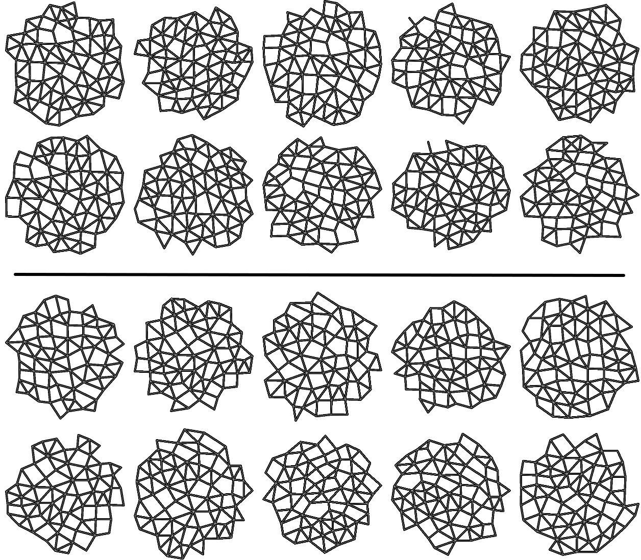
We take 20 confocal microscope images (13 from wild-type plants and 7 from trm678 mutants) of shoot apical meristems, and process them to extract graphs representing local neighborhoods of cells. Each graph consists of a cell and its 63 closest neighbors (64 cells total). Cell neighborhood selection was limited to the central region of each SAM image, since the primordia surrounding the SAM are known to have different morphological properties. For each cell neighborhood, we produce a graph by connecting two cells iff their shared boundary is 30 pixels or longer. For each edge, we save the length of this shared boundary, as well as the angle of the edge from horizontal and the edge length. We extracted 600 cell neighborhoods for each type, for a total of 1200 graphs. See Figure [fig:cell_lines] for an example SAM image and resulting graph, and see Figure [fig:cell_extracted].


[fig:cell_lines]
[fig:cell_extracted]
Species in the plant genus Arabidopsis are of high interest in plant morphology studies, owing to the facts that 1) its genome was fully sequenced in 1996, relatively early (Kaul et al. 2000), and 2) its structure makes it relatively easy to capture images of the area of active cell division: the shoot apical meristem (SAM). Cell-scale interaction of microtubules (as described in Chapter 7) and microtubule bundles are thought to influence the orientation of cell division planes in the SAM, and thereby influence the morphology of the organism as a whole. However, this connection is not yet entirely well-understood. Recent work (Dumais 2009; Schaefer et al. 2017) has found that mutations which decrease the level of expression of genes TRM6,TRM7,and TRM8 inhibit the formation of the preprophase band (PPB). Arabidopsis mutants with inhibited PPB formation demonstrate more variance in the placement of new cell walls during cell division.
Dataset
The dataset used in this analysis was prepared as follows:
Two varieties of Arabidopsis (wild type as well as “trm678 mutants”: mutants with decreased expression of all three of TRM6,TRM7,and TRM8) were planted and kept in the short-day condition (8 hours of light, 16 hours of dark) for 6 weeks.
Plants were transferred to long-day conditions and kept there until the SAM had formed. This took two weeks for wild-type plants and three weeks for TRM678 mutants.
The SAM of each pant was then was then dissected and observed with a confocal microscope, Leica SP8 upright scanning confocal microscope equipped with a water immersion objective (HC FLUOTAR L 25x/0.95 W VISIR).
This resulted in 3D images of the SAM from above (e.g. perpendicular to the plane of cell division) collected for both types of specimens.
Each 3D image was converted to a 2D image showing only the cell wall of the top layer of cells in the SAM.
Each image was segmented into individual cells, by finding connected components separated by cell walls.
Each segmented image was used to produce several graphs: a cell and its 63 nearest neighbors were taken as vertices (so that each graph had 64 vertices total). Vertices were connected if their corresponding cells shared a cell wall. We will refer to the resulting graph as a “morphological graph". Only cells which were within 128 pixels of the center of the image were used, to ensure that each morphological graph was only composed of cells in the central region of the SAM. This is important because cell morphology is radically different at the boundary between the SAM and the surrounding primordia. See Figure [fig:cell_images] for examples of cell segmentations and extracted graphs.
This procedure produced a population of 1062 morphological graphs of 64 vertices each: 513 graphs coming from wild-type cell images, and 549 graphs coming from trm678 mutants. See Figure [fig:cell_lines] for examples. Graph Diffusion Distance was used to compute a distance matrix comparing each pair of graphs. Figure [fig:cell_line_embeddings] shows an embedding of these distances, produced by plotting each point according to its projection onto the first two principal components of the distance matrix. This technique, multidimensional scaling (MDS), produces a 2D embedding such that inter-point distances in the embedding are as close as possible to those in the original distance matrix. We see that GDD appears to detect a trend: the embedding shows a clear clustering of each type of cell with cells of the same type.


[fig:cell_images]
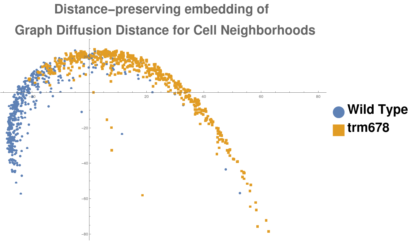
[fig:cell_line_embeddings]
Introduction
Graph Diffusion Distance (GDD) is a measure of similarity between graphs originally introduced by Hammond et. al (Hammond, Gur, and Johnson 2013) and greatly expanded by Scott et. al (C. Scott and Mjolsness 2021). This metric measures the similarity of two graphs by comparing their respective spectra. However, it is well-known that there exist pairs of cospectral graphs which are not isomorphic but have identical spectra. Furthermore, because even a small change to entries of a matrix may change its eigenvalues, another limitation of GDD is that it is sensitive to small changes in the topology of the graph (as well as small variations in edge weights). Finally, since GDD does not make use of edge or node attributes, it cannot distinguish between two different signals on the same source graph, diminishing its applicability in data science. In this work, we provide several generalizations to GDD which resolve these issues and make it a powerful machine learning tool for graphs.
Graph Diffusion Distance
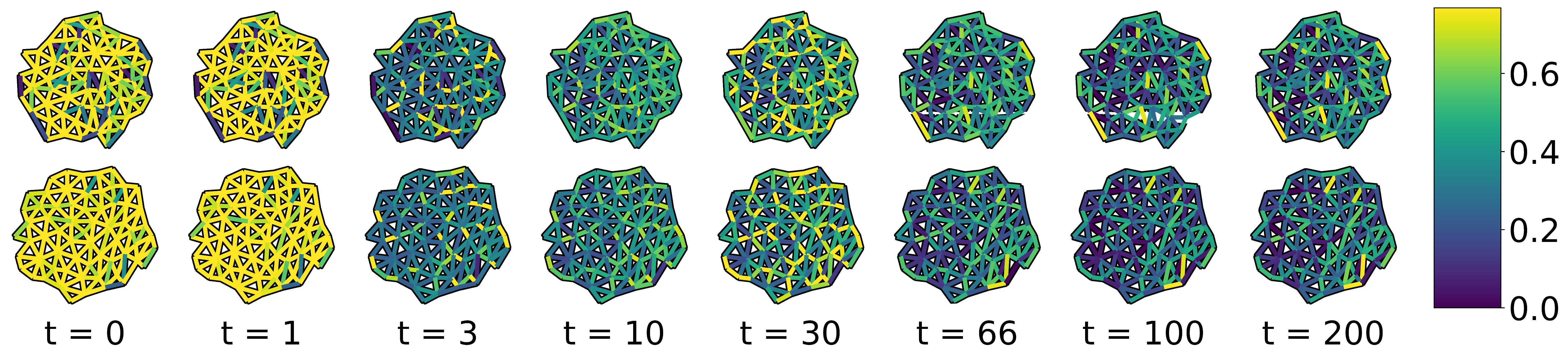
We use the definition of Graph Diffusion Distance (GDD) first given by Hammond et. al and later expanded (to cover differently-sized graphs) by Scott et. al. Given two graphs and , let and be their respective graph Laplacians. Furthermore, let be the diagonalizations of each Laplacian, so that is a diagonal matrix whose th diagonal entry, , is the th eigenvalue of . Then the graph diffusion distance between these graphs is given by This simplification relies on several properties of the Frobenius norm and the exponential map (rotation invariance and continuity, respectively) which we shall not detail here. It is clear that this distance measure requires the two graphs to be the same size, since otherwise this matrix difference is not defined.
GDD is a differentiable function of and edge weights
Once all of the eigenvalues and eigenvectors (of a matrix ) are computed, we may backpropagate through the eigendecomposition as described in (Nelson 1976) and (Andrew, Chu, and Lancaster 1993). If our edge weights (and therefore the values in the Laplacian matrix ) are parametrized by some value , and our loss function is dependent on the eigenvalues of , then we can collect the gradient as: In practice, if the entries of are computed as a function of using an automatic differentiation package (such as PyTorch (Paszke et al. 2019)) the gradient matrix is already known before eigendecomposition. We note here that for any fixed value of , all of the operations needed to compute GDD are either simple linear algebra or continuous or both. Therefore, for any loss function which takes the GDD between two graphs as input, we may optimize by backpropagation through the calculation of GDD using Equation [eqn:derivative_eigen].
Weighted Diffusion Distance
We make two main changes to GDD to make it capable of being tuned to specific graph data. First, we replace the real-valued optimization over with a maximum over an explicit list of values . This removes the need for an optimization step inside the GDD calculation. Second, we re-weight the Frobenius norm in the GDD calculation with a vector of weights which is the same length as the list of eigenvalues (these weights are normalized to sum to 1). The resulting GDD calculation is then: This distance calculation may then be explicitly included in the computation graph (e.g. in PyTorch) of a machine learning model, without needing to invoke some external optimizer to find the supremum over all . and may be tuned by gradient descent or some other optimization algorithm to minimize a loss function which takes as input. Tuning the values results in a list of values of for which GDD is most informative for a given dataset, while tuning reweights GDD to pay most attention to the eigenvalues which are most discriminative. In the experiments in Section [sec:numeric] we demonstrate the efficacy of tuning these parameters using contrastive loss.
Learning Edge Weighting Functions
Here, we note that if graph edge weights are determined by some function parametrized by , we may still apply all of the machinery of Sections 8.4.1 and 8.4.2. A common edge weighting function for graphs embedded in Euclidean space is the Gaussian Distance Kernel, , where is the distance between nodes and in the embedding. is the ‘radius’ of the distance kernel and can be tuned in the same way as and . In cases like the data discussed in this section, our edge weights are vector-valued, and it is therefore advantageous to replace this hand-picked edge weight with weights chosen by a general function approximator, e.g. an artificial neural network (Fukushima and Miyake 1982). As before, the parameters of this ANN could be tuned using gradients backpropagated through the GDD calculation and eigendecomposition. Example weights learned by an ANN, trained with the constrastive loss function, can be seen in Figure [fig:learned_edge_weights].
[fig:learned_edge_weights]
Numeric Experiments
Data Description
In this brief section we describe the two datasets used in preparation of this manuscript. For more details, please see the README accompanying each dataset.
Skeletonized MNIST
As another comparison, we try our method on graphs representing skeletonized images from the MNIST dataset. 300 MNIST digits from each category (3000 total) were selected at random. Each MNIST digit was converted into a skeleton using the skeletonize method from sklearn(Pedregosa et al. 2011), with default parameters. Each skeleton was then converted into the nearest-neighbors graph of live pixels. Finally, each graph was reduced to 32 nodes by randomly contracting neighboring nodes (excluding nodes which were endpoints or junctions). A vector-valued edge label was saved for each edge, including the angle of that edge from horizontal and the length of the edge. The dataset used in this section was prepared as follows:
Two varieties of Arabidopsis (wild type as well as “trm678 mutants”: mutants with decreased expression of all three of TRM6,TRM7,and TRM8) were planted and kept in the short-day condition (8 hours of light, 16 hours of dark) for 6 weeks.
Plants were transferred to long-day conditions and kept there until the SAM had formed. This took two weeks for wild-type plants and three weeks for TRM678 mutants.
The SAM of each pant was then was then dissected and observed with a confocal microscope, Leica SP8 upright scanning confocal microscope equipped with a water immersion objective (HC FLUOTAR L 25x/0.95 W VISIR).
This resulted in 3D images of the SAM from above (e.g. perpendicular to the plane of cell division) collected for both types of specimens.
Each 3D image was converted to a 2D image showing only the cell wall of the top layer of cells in the SAM.
Each image was segmented into individual cells, by finding connected components separated by cell walls.
Each segmented image was used to produce several graphs: a cell and its 63 nearest neighbors were taken as vertices (so that each graph had 64 vertices total). Vertices were connected if their corresponding cells shared a cell wall. We will refer to the resulting graph as a “morphological graph". Only cells which were within 128 pixels of the center of the image were used, to ensure that each morphological graph was only composed of cells in the central region of the SAM. This is important because cell morphology is radically different at the boundary between the SAM and the surrounding primordia. See Figure [fig:cell_images] for examples of cell segmentations and extracted graphs.
This procedure produced a population of 580 morphological graphs of 64 vertices each: 290 graphs coming from wild-type cell images, and 290 graphs coming from trm678 mutants. See Figure [fig:cell_lines] for example segmented images and an example graph. [sec:numeric] We test each of the GDD generalizations proposed, on each dataset. Both datasets were split 85/15 % train/validation; All metrics we report are calculated on the validation set. For each dataset, we compare the following four methods: 1) GDD on unweighted graphs, with no tuning of or other parameters; 2) Gaussian kernel edge weights (fixed ), with and tuned; 3) Gaussian kernel edge weights, with , , and 4) General edge weights parametrized by a small neural network. For methods 2 and 3, the input to the distance kernel was the distance between nodes in the original image. All parameters were tuned using ADAMOpt (Kingma and Ba 2014) (with default PyTorch hyperparameters and batch size 256) to minimize the contrastive loss function (Hadsell, Chopra, and LeCun 2006). Training took 200 epochs. For the neural network approach, edge weights were chosen as the final output of a neural network with three layers of sizes with SiLU activations on the first two layers and no activation function on the last layer. Results of these experiments can be found in Table [tab:valid_results_morpho], and distance matrices (along with a distance-preserving embedding (Cox and Cox 2008) of all points in the dataset) for the cell morphology dataset can be seen in Figure [fig:embedding_of_graphs]. The distance matrices developed using the ANN approach clearly show better separation between the two categories. The validation accuracy on the cell morphology dataset is best for the ANN method.
![Top row: distance matrices between cell morphology graphs produced using our methods 1-4, as described in Section [sec:numeric]. Bottom row: the result of embedding each distance matrix in 2D using its first two principal components. Training dataset points are semitransparent, validation points are opaque. Note: the principal components used for this embedding are calculated only on the submatrix which corresponds to training data.](../media/file65.png "fig:")
![Top row: distance matrices between cell morphology graphs produced using our methods 1-4, as described in Section [sec:numeric]. Bottom row: the result of embedding each distance matrix in 2D using its first two principal components. Training dataset points are semitransparent, validation points are opaque. Note: the principal components used for this embedding are calculated only on the submatrix which corresponds to training data.](../media/file66.png "fig:")
![Top row: distance matrices between cell morphology graphs produced using our methods 1-4, as described in Section [sec:numeric]. Bottom row: the result of embedding each distance matrix in 2D using its first two principal components. Training dataset points are semitransparent, validation points are opaque. Note: the principal components used for this embedding are calculated only on the submatrix which corresponds to training data.](../media/file67.png "fig:")
![Top row: distance matrices between cell morphology graphs produced using our methods 1-4, as described in Section [sec:numeric]. Bottom row: the result of embedding each distance matrix in 2D using its first two principal components. Training dataset points are semitransparent, validation points are opaque. Note: the principal components used for this embedding are calculated only on the submatrix which corresponds to training data.](../media/file68.png "fig:")
![Top row: distance matrices between cell morphology graphs produced using our methods 1-4, as described in Section [sec:numeric]. Bottom row: the result of embedding each distance matrix in 2D using its first two principal components. Training dataset points are semitransparent, validation points are opaque. Note: the principal components used for this embedding are calculated only on the submatrix which corresponds to training data.](../media/file69.png "fig:")
![Top row: distance matrices between cell morphology graphs produced using our methods 1-4, as described in Section [sec:numeric]. Bottom row: the result of embedding each distance matrix in 2D using its first two principal components. Training dataset points are semitransparent, validation points are opaque. Note: the principal components used for this embedding are calculated only on the submatrix which corresponds to training data.](../media/file70.png "fig:")
![Top row: distance matrices between cell morphology graphs produced using our methods 1-4, as described in Section [sec:numeric]. Bottom row: the result of embedding each distance matrix in 2D using its first two principal components. Training dataset points are semitransparent, validation points are opaque. Note: the principal components used for this embedding are calculated only on the submatrix which corresponds to training data.](../media/file71.png "fig:")
![Top row: distance matrices between cell morphology graphs produced using our methods 1-4, as described in Section [sec:numeric]. Bottom row: the result of embedding each distance matrix in 2D using its first two principal components. Training dataset points are semitransparent, validation points are opaque. Note: the principal components used for this embedding are calculated only on the submatrix which corresponds to training data.](../media/file72.png "fig:")
[fig:embedding_of_graphs]
| Method | Validation Accuracy % (morpho) |
|---|---|
| GDD only | 77.7 |
| -tuning and -weights | 85.0 |
| and -tuning,-weights | 85.5 |
| ANN Parametrization | 98.3 |
[tab:valid_results_morpho]
Conclusion and Future Work
This section presents two applications of GDD to the classification of graphs embedded in 2D and 3D. In both, we demonstrate that GDD (and a parametrized variant) produce clusters which draw out structural differences in our dataset(s). Additionally, we demonstrate a method to compute distance metrics between edge-labelled graphs, in such a way as to respect class labels. This approach is flexible and can be implemented entirely in PyTorch, making it possible to learn a distance metric between graphs that were previously not able to be discriminated by Graph Diffusion Distance. In the future we hope to apply this method to more heterogenous graph datasets by including the varying-size version of GDD. We also note here that our neural network approach, as described, is not a Graph Neural Network in the sense described by prior works like (Kipf and Welling 2016; Bacciu et al. 2020), as there is no message-passing step. We expect message-passing layers to directly improve these results and hope to include them in a future version of differentiable GDD.