Application: Multiscale Neural Network Training

Previous chapters have explored the properties of Graph Diffusion Distance, as well as explained how to compute it efficiently. In this chapter, we use the $P$ matrices which are a byproduct of computing Graph Diffusion Distance to accelerate the process of training a neural network. This is accomplished by defining a network which operates on multiple spatial scales of the input data, with the mapping in between scales performed by pre- and post-multiplication with $P$ matrices. The final model shares some structural similarities with multigrid solvers for differential equations, which we discuss in the next section.

Prior Work

In this section, we discuss prior attempts to apply ideas from multigrid methods to neural network models. Broadly speaking, prior approaches to neural net multigrid can be categorized into two classes: (1) Neural network models which are “structurally multigrid”, i.e. are typical neural network models which make use of multiple scales of resolution; and (2) Neural network training processes which are hierarchical in some way, or use a coarsening-refinement procedure as part of the training process.

In the first class are approaches (Grais et al. 2017; Ke, Maire, and Yu 2016; Serban et al. 2017). Ke et al (Ke, Maire, and Yu 2016) implement a convolutional network in which convolutions make use of a multigrid-like structure similar to a Gaussian pyramid, with the motivation that the network will learn features at multiple scales of resolution. Grais et. al (Grais et al. 2017) define a convolution operation, inspired by multigrid methods, that convolves at multiple levels of resolution simultaneously. Serban et. al (Serban et al. 2017) demonstrate a recurrent neural network model which similarly operates in multiple levels of some scale space; but in this work the scale space is a space of aggregated language models (specifically, the differing scales are different levels of generality in language models - for example, topic models are coarsest, word models are finest, with document models somewhere in between). Common to all three of these approaches is that they make use of a modified neural net structure while leaving the training process unchanged, except that the network accepts multiresolution inputs.

In contrast, multilevel neural network models (Bakshi and Stephanopoulos 1993; Schroder 2017) in the second category present modified learning procedures which also use methodology similar to multilevel modeling. Reference (Bakshi and Stephanopoulos 1993) introduces a network which learns at coarse scales, and then gradually refines its decision making by increasing the resolution of the input space and learning “corrections” at each scale. However, that paper focuses on the capability of a particular family of basis functions for neural networks, and not on the capabilities of the multigrid approach. Reference (Schroder 2017) presents a reframing of the neural network training process as an evolution equation in time, and then applies a method called MGRIT (Multigrid Reduction in Time (Falgout et al. 2014)) to achieve the same results as parallelizing over many runs of training.

Our approach is fundamentally different: we use coarsened versions of the network model to make coarse updates to the weight variables of our model, followed by ‘smoothing steps’ in which the fine-scale weights are refined. This approach is more general than any of (Grais et al. 2017; Ke, Maire, and Yu 2016; Serban et al. 2017), since it can be applied to any feed-forward network and is not tied to a particular network structure. The approach in (Schroder 2017) is to parallelize the training process by reframing it as a continuous-in-time evolution equation, but it still uses the same base model and therefore only learns at one spatial scale.

Our method is both structurally multilevel and learns using a multilevel training procedure. Our hierarchical neural network architecture is the first to learn at all spatial scales simultaneously over the course of training, transitioning between neural networks of varying input resolution according to standard multigrid method schedules of coarsening and refinement. To our knowledge, this represents a fully novel approach to combining the powerful data analysis of neural networks with the model acceleration of multiscale modeling.

Outline

Building on the terminology in Chapters 1 and 2, in Section 6.2 we define an objective function which evaluates a map between two graphs, in terms of how well it preserves the behavior of some local process operating on those graphs (interpreting the smaller of the two graphs as a coarsened version of the larger). This is the core theory of this chapter: that of optimal prolongation maps between computational processes running on graph-based data structures, and hence between graphs. In this chapter we use a specific example of such a process, single-particle diffusion on graphs, to examine the behavior of these prolongation maps. Finally, we discuss numerical methods for finding (given two input graphs $G_1$ and $G_2$ , and a process) prolongation and restriction maps which minimize the error of using $G_1$ as a surrogate structure for simulating the behavior of that process on $G_2$ . We will define more rigorously what we mean by “process”, “error”, and “prolongation” in Section 6.2. In Subsection 6.3.2 we examine some properties of this objective function, including presenting some projection matrices which are local optima for particular choices of graph structure and process. In Subsections 6.4 and 6.4.2, we define the Multiscale Artificial Neural Network (MsANN), a hierarchically-structured neural network model which uses these optimized projection matrices to project network parameters between levels of the hierarchy, resulting in more efficient training. In Section 6.5, we demonstrate this efficiency by training a simple neural network model on a variety of datasets, comparing the cost of our approach to that of training only the finest network in the hierarchy.

Optimal Prolongation Maps Between Graphs

Given two graphs $G_1$ and $G_2$ , we find the optimal prolongation map between them as follows: We first calculate the graph Laplacians $L_1$ and $L_2$ , as well as pairwise vertex Manhattan distance matrices (i.e. the matrix with $T_{i,j}$ the minimal number of graph edges between vertices $i$ and $j$ in the graph), $T_1$ and $T_2$ , of each graph. Calculating these matrices may not be trivial for arbitrary dense graphs; for example, calculating the pairwise Manhattan distance of a graph with $m$ edges on $n$ vertices can be accomplished in $O(m + n \log n)$ by the Fibonacci heap version of Dijkstra’s algorithm (Fredman and Tarjan 1987). Additionally, in Section $\ref{sec:optresults}$ we discuss an optimization procedure which requires computing the eigenvalues of $L_i$ (which are referred to as the spectrum of $G_i$ ). Computing graph spectra is a well studied problem; we direct the reader to (Cohen-Steiner et al. 2018; Pan and Chen 1999). In practice, all of the graph spectra computed for experiments in this chapter took a negligible amount of time ( $<$ 1s) on a modern consumer-grade laptop using the scipy.linalg package (Jones et al., n.d.), which in turn uses LAPACK routines for Schur decomposition of the matrix (Anderson et al. 1999). The optimal map is defined as $P$ which minimizes the matrix function $$\begin{aligned} \label{eqn:objfunction} & \inf_{P | C(P), \alpha > 0, \beta > 0} && E(P) \hfill & \\ = & \inf_{P | C(P), \alpha > 0, \beta > 0} && \left[ (1-s) {\left| \left| \frac{1}{\sqrt{\alpha}} P L_1 - \sqrt{\alpha} L_2 P \right|\right|}^2_F \right. & \text{``Diffusion Term"} \nonumber \\ & && \left. + s {\left|\left|\frac{1}{\sqrt{\beta}} P T_1 - \sqrt{\beta} T_2 P \right| \right|}^2_F \right] & \text{``Locality Term"\footnotemark} \nonumber \end{aligned}$$ where $|| \cdot ||_F$ is the Frobenius norm, and $C(P)$ is a set of constraints on $P$ (in particular, we require $P^T P = I_{n_1}$ , but could also impose other restrictions such as sparsity, regularity, and/or bandedness). The manifold of real-valued orthogonal $n_2 \times n_1$ matrices with $n_1 \leq n_2$ is known as the Stiefel manifold; minimization constrained to this manifold is a well-studied problem (Rapcsák 2002; Turaga, Veeraraghavan, and Chellappa 2008). This optimization problem can be thought of as measuring the agreement between processes on each graph, as mapped through $P$ . The expression $P X_1 - X_2 P$ compares the end result of

Advancing process $X_2$ forward in time on $G_2$ and then using $P$ to interpolate vertex states to the smaller graph, to:
Interpolating the initial state (the all-ones vector) using $P$ and then advancing process $X_1$ on $G_1$ .

Strictly speaking the above interpretation of our objective function does not apply to the Manhattan distance matrix T of a graph, since $T$ is not a valid time evolution operator and thus is not a valid choice for $X$ . However, the objective function term containing $T$ may still be interpreted as comparing travel distance in one graph to travel distance in the other. That is, we are implicitly comparing the similarity of two ways of measuring the distance of two nodes $v_k$ and $v_l$ in $G_1$ :

The Manhattan distance, as defined above, and;
$\sum_{i = 1}^{n_2} \sum_{j = 1}^{n_2} p_{ik} d_{G_2}(u_i, u_j) p_{jl}$ , a sum of path distances in $G_2$ weighted by how strongly $v_k$ and $v_l$ are connected, through $P$ , to the endpoints of those paths, $u_i$ and $u_j$ .

Parameters $\alpha$ and $\beta$ are rescaling parameters to compensate for different graph sizes; in other words, $P$ must only ensure that processes 1 and 2 above agree up to some multiplicative constant. In operator theory terminology, the Laplacian is a time evolution operator for the single particle diffusion equation: $L_i = A(G_i) - \text{diag}(1 \cdot A(G_i))$ . This operator evolves the probability distribution of states of a single-particle diffusion process on a graph $G_i$ (but other processes could be used - for example, a chemical reaction network or multiple-particle diffusion). The process $L$ defines a probability-conserving Master Equation of nonequilibrium statistical mechanics $dp/dt = L \cdot p$ which has formal solution $p(t) = \exp{(t L)} \cdot p(0)$ . Pre-multiplication by the prolongation matrix $P$ is clearly a linear operator i.e. linear transformation from $\mathbb{R}^{n_1}$ to $\mathbb{R}^{n_2}$ . Thus, we are requiring $P$ which minimizes the degree to which the operator diagram

$$\begin{diagram} L_1 &\rTo^{\Delta t} & {L_1}'\\ \dTo_{P} & &\dTo_{P} &&&& (\text{Diagram }1) \\ L_2 &\rTo^{\Delta t} & {L_2}'\\ \end{diagram}$$ fails to commute. $\Delta t$ of course refers to advancement in time. See (Johnson et al. 2015), Figure 1, for a more complete version of this commutative diagram for model reduction.

We thus include in our objective function terms with 1) graph diffusion and 2) graph locality as the underlying process matrices ( $T$ , the Manhattan distance matrix, cannot be considered a time evolution operator because it is not probability-preserving). Parameter $s$ adjusts the relative strength of these terms to each other; so we may find “fully diffuse” $P$ when $s = 0$ and “fully local” $P$ when $s = 1$ . Figure [fig:localityfig] illustrates this tradeoff for an example prolongation problem on a pair of grid graphs, including the transition from a global optimum of the diffusion term to a global optimum of the locality term. In each case, we only require $P$ to map these processes into one another up to a multiplicative constant: $\alpha$ for the diffusion term and $\beta$ for the locality term. Exhaustive grid search over $\alpha$ and $\beta$ for a variety of prolongations between (a) path graphs and (b) 2D grid graphs of varying sizes has suggested that for prolongation problems where the $G_i$ are both paths or both grids, the best values (up to the resolution of our search, $10^{-6}$ ) for these parameters are $\alpha=1.0$ and $\beta=n_1/n_2$ . However, we do not expect this scaling law to hold for general graphs.

Figure 1: Several solutions of our objective function found by PyManOpt as s, the relative weight of the two terms of our objective function, is tuned from 0 (fully diffuse, top left) to 1 (fully local, bottom right). Within each subplot, grayscale indicates the magnitude of matrix entries. Note that the P matrices found with s=0 do not appear to be structured in a way which respects the locality of the original graphs, whereas the matrices with s=1 do. — Figure 1: Several solutions of our objective function found by PyManOpt as $s$ , the relative weight of the two terms of our objective function, is tuned from 0 (fully diffuse, top left) to 1 (fully local, bottom right). Within each subplot, grayscale indicates the magnitude of matrix entries. Note that the $P$ matrices found with $s=0$ do not appear to be structured in a way which respects the locality of the original graphs, whereas the matrices with $s=1$ do.

Comparison of Numerical Methods

[sec:optresults]

To find minima of this objective function, we explore several numerical methods. For prototyping, we initially used Nelder-Mead (Nelder and Mead 1965) optimization with explicit orthogonality constraints, as implemented in the Mathematica commercial computer algebra program. However, this approach does not scale - in our hands Mathematica was not able to minimize this objective function with more than approximately $200$ unknowns in a reasonable amount of time. Our next approach was to use a special-purpose code (Wen and Yin 2013) for orthogonally-constrained gradient descent. While this software package scaled well to pairs of large graphs, it required many random restarts to find minima of our objective function. Motivated by its automatic differentiation capability and its ability to handle larger numbers of unknowns, we tried the TensorFlow minimization package (Abadi et al. 2016): first custom-written code and then a package called PyManOpt (Townsend, Koep, and Weichwald 2016) which performs manifold-constrained optimization of arbitrary objective functions expressed as TensorFlow computation graphs. PyManOpt is able to perform first- and second-order minimization while staying within the constraint manifold (rather than our custom code, which takes gradient descent steps and then projects back to the constraint surface). These latter two approaches performed best in terms of optimization solution quality, and we compare them more throughly below.

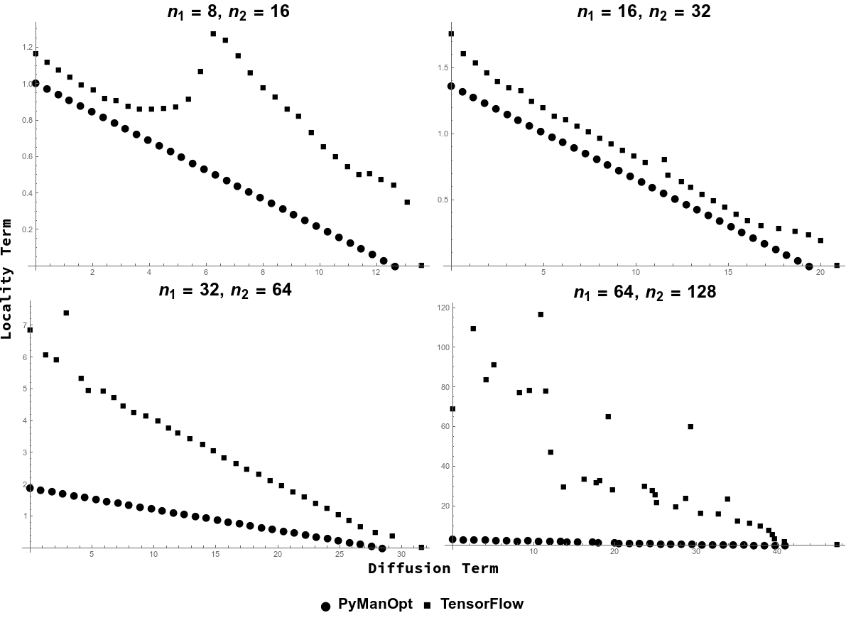
To compare the performance of the TensorFlow method and the PyManOpt method, we explore the performance of both minimization methods as the relative weight $s$ of the locality and diffusion terms is adjusted. Figure [fig:paretofig] shows the tradeoff plot of the optimized unweighted value of each term as the weight parameter $s$ is tuned. The four subplots correspond to four runs of this experiment with differing sizes of graphs; in each we find optimal prolongations from a cycle graph of size $n$ to one of size $2n$ . The PyManOpt-based minimization code is clearly superior, as we see a clear linear tradeoff between objective function terms as a function of $s$ . The TensorFlow code which maintains orthogonality by projecting back to the Stiefel manifold falls short of this boundary in all cases. Therefore unless otherwise specified, for the rest of this chapter when we discuss solving for $P$ matrices, we are reporting results of using the PyManOpt method.

Figure 2: Tradeoff plot of locality vs. diffusion for several pairs of graphs. Multiple solutions are plotted in each subplot, representing the adjustment of the s parameter in our objective function from totally local to totally diffuse. We see that the PyManOpt boundary shows a linear tradeoff between the two terms of the objective function as their relative weight is tuned, whereas the Tensorflow boundary is more irregular. Furthermore, the PyManOpt method in general finds optima with lower objective function value than Tensorflow (for both objectives). We note that Nelder-Mead in Mathematica would not be able to tackle problems of this size, and the method due to Wen and Yin (Wen and Yin 2013) produced points which are off of this plot by at least an order of magnitude (we do not present these points). — Figure 2: Tradeoff plot of locality vs. diffusion for several pairs of graphs. Multiple solutions are plotted in each subplot, representing the adjustment of the $s$ parameter in our objective function from totally local to totally diffuse. We see that the PyManOpt boundary shows a linear tradeoff between the two terms of the objective function as their relative weight is tuned, whereas the Tensorflow boundary is more irregular. Furthermore, the PyManOpt method in general finds optima with lower objective function value than Tensorflow (for both objectives). We note that Nelder-Mead in Mathematica would not be able to tackle problems of this size, and the method due to Wen and Yin (Wen and Yin 2013) produced points which are off of this plot by at least an order of magnitude (we do not present these points).

Initialization

We initialize our minimization with an upper-bound solution given by the Munkres minimum-cost matching algorithm; the initial $P$ is $m^*(L_1, L_2)$ as defined in equation [eqn:matchingconstraints], i.e. the binary matrix where an entry $P_{(i,j)}$ is 1 if the pair $(i,j)$ is one of the minimal-cost pairs selected by the minimum-cost assignment algorithm, and 0 otherwise. While this solution is, strictly speaking, minimizing the error associated with mapping the spectrum of one graph into the spectrum of the other (rather than actually mapping a process running on one graph into a process on the other) we found it to be a reasonable initialization, outperforming both random restarts and initialization with the appropriately sized block matrix $\left( \begin{array}{c} I \\ 0 \end{array}\right)$ .

Precomputing $P$ matrices

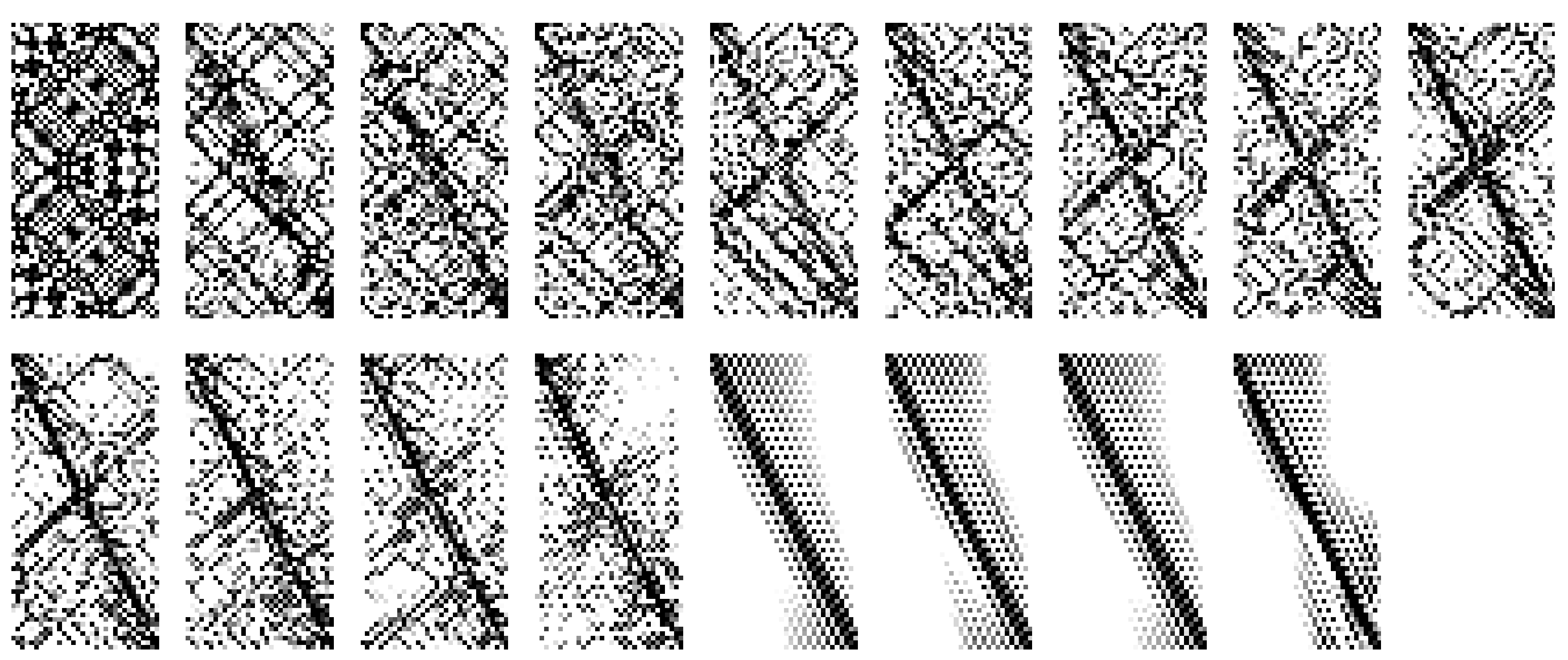
For some structured graph lineages it may be possible to derive formulaic expressions for optimal $P$ and $\alpha$ , as a function of the lineage index. For example, during our experiments we discovered species of $P$ which are local minima of prolongation between path graphs, cycle graphs, and grid graphs. A set of these outputs is shown in Figure [fig:localityfig]. They feature various diagonal patterns as naturally idealized in Figure [fig:pspeciesfig]. These idealized versions of these patterns all are also empirical local minima of our optimization procedure, for $s=0$ or $s=1$ , as indicated. Each column of Figure [fig:pspeciesfig] provides a regular family of $P$ structures for use in our subsequent experiments in Section 6.5. We have additionally derived closed-form expressions for global minima of the diffusion term of our objective function for some graph families (cycle graphs and grid graphs with periodic boundary conditions). However, in practice these global minima are nonlocal (in the sense that they are not close to optimizing the locality term) and thus may not preserve learned spatial rules between weights in levels of our hierarchy.

Examples of these formulaic $P$ matrices can be seen in Figure [fig:pspeciesfig]. Each column of that figure shows increasing sizes of $P$ generated by closed-form solutions which were initially found by solving smaller prolongation problems (for various graph pairs and choices of $s$ ) and generalizing the solution to higher $n$ . Many of these examples are similar to what a human being would design as interpolation matrices between cycles and periodic grids. However, (a) they are valid local optima found by our optimization code and (b) our approach generalizes to processes running on more complicated or non-regular graphs, for which there may not be an obvious a priori choice of prolongation operator.

We highlight the best of these multiple species of closed-form solution, for both cycle graphs and grid graphs. The interpolation matrix-like $P$ seen in the third column of the “Cycle Graphs" section, or the sixth column of the “Grid Graphs” section of Figure [fig:pspeciesfig], were the local optima with lowest objective function value (with $s = 1$ , i.e. they are fully local). As the best optima found by our method(s), these matrices were our choice for line graph and grid graph prolongation operators in our neural network experiments, detailed in Section 6.5. We reiterate that in those experiments we do not find the $P$ matrices via any optimization method - since the neural networks in question have layer sizes of order $10^3$ , finding the prolongation matrices from scratch may be computationally difficult. Instead, we use the solutions found on smaller problems as a recipe for generating prolongation matrices of the proper size.

Furthermore, given two graph lineages $G_1^{(1)}, G_1^{(2)}, G_1^{(3)} \ldots$ and $G_2^{(1)}, G_2^{(2)}, G_2^{(3)} \ldots$ , and sequences of optimal matrices $P_1^{(1)}, P_1^{(2)}, P_1^{(3)} \ldots$ and $P_2^{(1)}, P_2^{(2)}, P_2^{(3)} \ldots$ mapping between successive members of each, we can construct $P$ which are related to the optima for prolonging between members of a new graph lineage which is comprised of the levelwise graph box product of the two sequences. We show in (Section 3.5, Corollary [thm:decompcorollary]) conditions under which the value of the objective function at $P_{\text{box}}^{(i)} = P_1^{(i)} \otimes P_2^{(i)}$ is an upper bound of the optimal value for prolongations between members of the lineage $G_1^{(1)} \Box G_2^{(1)}, G_1^{(2)} \Box G_2^{(2)}, G_1^{(3)} \Box G_2^{(3)}, \ldots$ . We leave open the question of whether such formulaic $P$ exist for other families of structured graphs (complete graphs, $k$ -partite graphs, etc.). Even in cases where formulaic $P$ are not known, the computational cost of numerically optimizing over $P$ may be amortized, in the sense that once a $P$ -map is calculated, it may be used in many different hierarchical neural networks or indeed many different multiscale models.

Multiscale Artificial Neural Network Algorithm

In this section we describe the Multiscale Artificial Neural Network (MsANN) training procedure, both in prose and in pseudocode (Algorithm [alg:mgannalg]). Let $\mathcal{M}_0 \ldots \mathcal{M}_{L}$ be a sequence of neural network models with identical “aspect ratios” (meaning the sizes of each layer relative to other layers in the same model) but differing input resolution, so that $\mathcal{M}_0$ operates at the finest scale and $\mathcal{M}_L$ at the coarsest. For each model $\mathcal{M}_l$ , let $\theta^{(l)}_0, \theta^{(l)}_1, \ldots \theta^{(l)}_{n_\text{vars}-1}$ be a list of the $n_\text{vars}$ network parameters (each in matrix or vector form) in some canonical order which is maintained across all scales. Let the symbol $\mathcal{P}^{(l)}_j$ represent either:

If the network parameters $\theta^{(i)}_j$ at levels $i = 0 \ldots L$ are weight matrices between layers $m_1$ and $m_2$ of each hierarchy, then $\mathcal{P}^{(l)}_j$ represents a pair of matrices $\left( P^{(l)}_{\text{input}_j}, P^{(l)}_{\text{output}_j} \right)$ , such that:
- $P^{(l)}_{\text{input}_j}$ prolongs or restricts between possible values of nodes in layer $m_1$ of model $\mathcal{M}_l$ , and values of nodes in layer $m_1$ of model $\mathcal{M}_{l+1}$ .
- $P^{(l)}_{\text{output}_j}$ does the same for possible values of nodes in layer $m_2$ of each model.
If the network parameters $\theta^{(i)}_j$ at levels $i = 0 \ldots L$ are bias vectors which are added to layer $m$ of each hierarchy, then $\mathcal{P}^{(l)}_j$ represents a single $P^{(l)}_j$ which prolongs or restricts between possible values of nodes in layer $m$ of model $\mathcal{M}_l$ , and values of nodes in layer $m$ of model $\mathcal{M}_{l+1}$ .

As a concrete example, for a hierarchy of single-layer networks $\mathcal{M}_0, \mathcal{M}_1, \mathcal{M}_2$ , each with one weight matrix $W^{(l)}$ and one bias vector $b^{(l)}$ , we could have $\theta^{(l)}_0 = W^{(l)}, \theta^{(l)}_1 = b^{(l)}$ for each $\mathcal{M}_l$ . $\mathcal{P}^{(0)}_0$ would represent a pair of matrices which map between the space of possible values of $W^{(0)}$ and the space of possible values of $W^{(1)}$ in a manner detailed in the next section. On the other hand, $\mathcal{P}^{(0)}_1$ would represent a single matrix which maps between $b^{(0)}$ and $b^{(1)}$ . Similarly, $\mathcal{P}^{(1)}_0$ would map between $W^{(1)}$ and $W^{(2)}$ , and $\mathcal{P}^{(1)}_1$ between $b^{(1)}$ and $b^{(2)}$ . In Section 6.4.2, we describe a general procedure for training such a hierarchy according to standard multilevel modeling schedules of refinement and coarsening, with the result that the finest network, informed by the weights of all coarser networks, requires fewer training examples.

Weight Prolongation and Restriction Operators

In this section we introduce the prolongation and restriction operators for neural network weight and bias optimization variables in matrix or vector form respectively.

For a 2D matrix of weights $W$ , define $\begin{gathered} \label{eqn:weightpro} \begin{aligned} \text{Pro}_{\mathcal{P}} \circ W &\equiv \text{Pro}_{(P_{\text{input}}, P_{\text{output}})} \circ W &\equiv P_{\text{input}} W P_{\text{output}}^T \\ % % \text{Res}_{\mathcal{P}} \circ W &\equiv \text{Res}_{(P_{\text{input}}, P_{\text{output}})} \circ W &\equiv P_{\text{input}}^T W P_{\text{output}} % % \end{aligned}\end{gathered}$ where $P_{\text{input}}$ and $P_{\text{output}}$ are each prolongation maps between graphs which respect the structure of the spaces of inputs and outputs of $W$ , i.e. whose structure is similar to the structure of correlations in that space. Further research is necessary to make this notion more precise. In our experiments on autoencoder networks in Section 6.5, we use example problems with an obvious choice of graph to use. In these 1D and 2D machine vision tasks, where we expect each pixel to be highly correlated with the activity of its immediate neighbors in the grid, 1D and 2D grids are clear choices of graphs for our prolongtion matrix calculation. Other choices may lead to similar results; for instance, we speculate that since neural network weight matrices may be interpreted as the weights of a multipartite graph of connected neurons in the network, these graphs could be an alternate choice of structure to prolong/restrict between. We leave for future work the development of automatic methods for determining these structures.

Note that the Pro and Res linear operators satisfy $\text{Res}_{\mathcal{P}} \circ \text{Pro}_{\mathcal{P}} = I$ , the identity operator, so $\text{Pro}_{\mathcal{P}} \circ \text{Res}_{\mathcal{P}}$ is a projection operator. We see in the experiment on mapping MNIST handwritten digits to a latent space (Subsection 6.5.2), for example, that if the input space has a high degree of 2D correlation between variables, but we use $P$ calculated between 1D path graphs, our multigrid procedure outlined below will sometimes fail to improve over training at only the finest scale. We hypothesize that this effect may be due to 1D prolongations discarding too much of the 2D correlation in the image data.

For a 1D matrix of biases $b$ , define $% \label{eqn:biaspro} \begin{split} % % \text{Pro}_{\mathcal{P}} \circ b &= P \cdot b \\ % % \text{Res}_{\mathcal{P}} \circ b &= P^T \cdot b % % % \end{split} %$ where, as before, we require that $P$ be a prolongation matrix between graphs which are appropriate for the dynamics of the network layer where $b$ is applied. Again $\text{Res}_{\mathcal{P}} \circ \text{Pro}_{\mathcal{P}} = I$ .

Given such a hierarchy of models $\mathcal{M}_0 \ldots \mathcal{M}_L$ , and appropriate and operators as defined above, we define a Multiscale Artificial Neural Network (MsANN) to be a neural network model with the same layer and parameter dimensions as the largest model in the hierarchy, where each layer parameter $\Theta_j$ is given by a sum of prolonged weight matrices from level $j$ of each of the models defined above: $$\begin{aligned} \label{eqn:hierarch_var_eqn} \Theta_j = \theta^{(0)}_j &+ \text{Pro}_{1 \rightarrow 0} \circ \theta^{(1)}_j + \text{Pro}_{2 \rightarrow 0} \circ \theta^{(2)}_j \ldots \text{Pro}_{L \rightarrow 0} \circ \theta^{(L)}_j \\ \intertext{Here we are using $\text{Pro}_{k \rightarrow 0}$ as a shorthand to indicate composed prolongation from model $k$ to model $0$, so if $\theta^{(i)}_j$ are weight variables we have (by Equation \ref{eqn:weightpro}) } \Theta_j = \theta^{(0)}_j &+ P^{(0)}_{\text{input}_j} \theta^{(1)}_j {\left( P^{(0)}_{\text{output}_j} \right)}^T \\ &+ P^{(0)}_{\text{input}_j} P^{(1)}_{\text{input}_j} \theta^{(2)}_j {\left( P^{(1)}_{\text{output}_j} \right)}^T {\left( P^{(0)}_{\text{output}_j} \right)}^T \nonumber \\ & + \quad \ldots \quad + \left( P^{(0)}_{\text{input}_j} \ldots P^{(L-1)}_{\text{input}_j} \theta^{(L)}_j {\left( P^{(L-1)}_{\text{output}_j} \right)}^T \ldots {\left( P^{(0)}_{\text{output}_j} \right)}^T \right) \nonumber \intertext{and if $\theta^{(i)}_j$ are bias variables we have (by Equation \ref{eqn:biaspro})} \Theta_j = \theta^{(0)}_j & + P^{(0)}_{\text{bias}_j} \theta^{(1)}_j + P^{(0)}_{\text{bias}_j} P^{(1)}_{\text{bias}_j} \theta^{(2)}_j + \ldots + \left( P^{(0)}_{\text{bias}_j} P^{(1)}_{\text{bias}_j} \ldots P^{(L-1)}_{\text{bias}_j} \theta^{(L)}_j \right)\end{aligned}$$ We note that matrix products such as $P^{(0)}_{\text{input}_j} \ldots P^{(k)}_{\text{input}_j}$ need only be computed once, during model construction.

Multiscale Artificial Neural Network Training

The Multiscale Artificial Neural Network algorithm is defined in terms of a recursive ‘cycle’ that is analogous to one epoch of default neural network training. Starting with $\mathcal{M}_0$ (i.e. the finest model in the hierarchy), we call the routine $\text{MsANNCycle}(0)$ , which is defined recursively. At any level $l$ , MsANNCycle trains the network at level $l$ for $k$ batches of training examples, recurses by calling $\text{MsANNCycle}(l + 1)$ , and then returns to train for $k$ further batches at level $l$ . The number of calls to $\text{MsANNCycle}(l + 1)$ inside each call to $\text{MsANNCycle}(l)$ is given by a parameter $\gamma$ .

This is followed by additional training at the refined scale; this process is normally (Vaněk, Mandel, and Brezina 1996) referred to by the multigrid methods community as ‘restriction’ and ‘prolongation’ followed by ‘smoothing’. The multigrid methods community additionally has special names for this type of recursive refining procedure with $\gamma = 1$ (“V-Cycles”) and $\gamma = 2$ (“W-Cycles”). See Figure [fig:gammafig] for an illustration of these contraction and refinement schedules. In our numerical experiments below, we examine the effect of this parameter on multigrid network training.

Neural network training with gradient descent requires computing the gradient of the error $E$ between the network output and target with regard to the network parameters. This gradient is computed by taking a vector of error for the nodes in the output layer, and backpropagating that error backward through the network layer by layer to compute the individual weight matrix and bias vector gradients. An individual network weight or bias term $w$ is then adjusted using gradient descent, i.e. the new value $w'$ is given by $w' = w - \eta \frac{d E}{d w}$ , where $\eta$ is a learning rate or step size. Several techniques can be used to dynamically change learning rate during model training - we refer the reader to (Bishop 2006) for a description of these techniques and backpropagation in general.

Our construction of the MsANN model above did not make use of the $\text{Res}$ (restriction) operator - we show here how this operator is used to compute the gradient of the coarsened variables in the hierarchy. This can be thought of as continuing the process of backpropagation through the $\text{Pro}$ operator. For these calculations we assume $\Theta_j$ is a weight matrix, and derive the gradient for a particular $\theta^{(k)}_j$ . For notational simplicity we rename these matrices $W$ and $V$ , respectively. We also collapse the matrix products $\begin{aligned} P^\text{(input)} &= P^{(0)}_{\text{input}_j} P^{(1)}_{\text{input}_j} \ldots P^{(k)}_{\text{input}_j} \\ {\left( P^\text{(output)} \right)}^T &= {\left( P^{(L-1)}_{\text{output}_j} \right)}^T {\left( P^{(L-2)}_{\text{output}_j} \right)}^T \ldots {\left( P^{(0)}_{\text{output}_j} \right)}^T\end{aligned}$ Let $\frac{d E}{d W}$ be a matrix where ${\left(\frac{d E}{d W} \right)}_{mn} = \frac{d E}{d w_{mn}}$ , calculated via backpropagation as described above. Then, for some $m,n$ : $\begin{aligned} \frac{d w_{mn}}{d v_{kl}} &= \frac{d }{d v_{kl}} {\left( \ldots + \text{Pro}_{} \circ V +\ldots \right)}_{mn} \\ &= \frac{d }{d v_{kl}} {\left( \ldots + \text{Pro}_{k \rightarrow 0} \circ V +\ldots \right)}_{mn} = \frac{d }{d v_{kl}} {\left( \text{Pro}_{k \rightarrow 0} \circ V \right)}_{mn} \nonumber \\ &= \frac{d }{d v_{kl}} {\left( P^\text{(input)} V {\left( P^\text{(output)} \right)}^T \right)}_{mn} = \frac{d }{d v_{kl}} \left( \sum_{a,b} p^\text{(input)}_{ma} v_{ab} p^\text{(output)}_{nb} \right) \nonumber \\ &= \left( p^\text{(input)}_{mk} p^\text{(output)}_{nl} \right) \nonumber \end{aligned}$ Then, $$\begin{aligned} \frac{d E}{d v_{kl}} &= \sum_{m,n} \frac{d E}{d w_{mn}} \frac{d w_{mn}}{d v_{kl}} \\ &= \sum_{m,n} \frac{d E}{d w_{mn}} p^\text{(input)}_{mk} p^\text{(output)}_{nl} \nonumber \\ &= {\left( {\left( P^\text{(input)} \right)}^T \frac{d E}{d W} P^\text{(output)} \right)_{kl}} \nonumber \\ \intertext{and so} \frac{d E}{d V} &= {\left( P^\text{(input)} \right)}^T \frac{d E}{d W} P^\text{(output)}\nonumber \\ \intertext{and therefore finally} \label{eqn:msann_res_equation} \frac{d E}{d V} &= \text{Res}_{0 \rightarrow k} \circ \frac{d E}{d W} \end{aligned}$$ where $\text{Res}$ is as in [eqn:weightpro].

We also note here that our code implementation of this procedure does not make explicit use of the $\text{Res}$ operator; instead, we use the automatic differentiation capability of Tensorflow (Abadi et al. 2016) to compute this restricted gradient. This is necessary because data is supplied to the model, and error is calculated, at the finest scale only. Hence we calculate the gradient at this scale and restrict it to the coarser layers of the model. It may be possible to feed coarsened data through only the coarser layers of the model, eliminating the need for computing the gradient at the finest scale, but we do not explore this method in this thesis.

Figure 3: Visits to models in a hierarchy of neural networks realized by several values of the recursion frequency parameter \gamma. The \gamma = 1 case and the \gamma = 2 case are referred to as “V-cycles” and “W-cycles”, respectively. Each time the multilevel training procedure visits a level, it performs some number, k, of smoothing steps (i.e. gradient descent at that resolution) at that model. — Figure 3: Visits to models in a hierarchy of neural networks realized by several values of the recursion frequency parameter $\gamma$ . The $\gamma = 1$ case and the $\gamma = 2$ case are referred to as “V-cycles” and “W-cycles”, respectively. Each time the multilevel training procedure visits a level, it performs some number, $k$ , of smoothing steps (i.e. gradient descent at that resolution) at that model.

Machine Learning Experiments

[subsec:mle_prelim] We present four experiments using this Multiscale Neural Network method. All of the experiments below demonstrate that our multigrid method outperforms default training (i.e. training only the finest-scale network), in terms of the number of training examples (summed over all scales) needed to reach a particular mean-squared error (MSE) value. We perform two experiments with synthetic machine vision tasks, as well as two experiments with benchmark image datasets for machine learning. While all of the examples presented here are autoencoder networks (networks whose training task is to reproduce their input at the output layer, while passing through a bottleneck layer or layers), we do not mean to imply that MsANN techniques are constrained to autoencoder networks. All network training uses the standard backpropagation algorithm to compute training gradients, and this is the expected application domain of our method. Autoencoding image data is a good choice of machine learning task for our experiments for two main reasons. First, autoencoders are symmetric and learn to reproduce their input at their output. Other ML models (for instance, neural networks for classification) have output whose nodes are not spatially correlated, and it is not yet clear if our approach will generalize to this type of model. Secondly, since the single and double-object machine vision tasks operate on synthetic data, we can easily generate an arbitrary number of samples from the data distribution, which was useful in the early development of this procedure. Our initial successes on this synthetic data led us to try the same task with a standard benchmark real-world dataset. For each experiment, we use the following measure of computational cost to compare relative performance. Let $\left| \mathcal{M} \right|$ be the number of trainable parameters in model $\mathcal{M}$ . We compute the cost of a training step of the weights in model $\mathcal{M}_k$ using a batch of size $b$ as $\frac{|\mathcal{M}_k|}{|\mathcal{M}_0|} b$ . The total cost $C(t)$ of training at step $t$ is the sum of this cost over all training steps thus far at all scales. This cost is motivated by the fact that the number of multiply operations for backpropagation is $O(n m)$ in the total number of network parameters $m$ and training examples $n$ , so we are adding up the relative cost of using a batch of size $b$ to adjust the weights in model $\mathcal{M}_k$ , as compared to the cost of using that same batch to adjust the weights in $\mathcal{M}_0$ .

Simple Machine Vision Task

As an initial experiment in the capabilities of hierarchical neural networks, we first try two simple examples: finding lower-dimensional representation of two artificial datasets. In both cases, we generate synthetic data by uniformly sampling from

the set of binary-valued vectors with one “object” comprising a contiguous set of pixels one-eighth as long as the entire vector set to 1, and the rest zero; and
the set of vectors with two such non-overlapping objects.

In each case, the number of possible unique data vectors is quite low: for inputs of size 1024, we have 1024 - 128 = 896 such vectors. Thus, for both of the synthetic datasets we add binary noise to each vector, where each “pixel" of the input has an independent chance of firing spuriously with $p=0.05$ . This noise in included only in the input vector, making these networks Denoising Autoencoders: models whose task is to remove noise from an input image.

Single-Object Autoencoder

We first test the performance of this procedure on a simple machine vision task. The neural networks in our hierarchy of models each have layer size specification (in number of units) $[2^n, 2^{n-2}, 2^{n-3} ,2^{n-2}, 2^n]$ for $n$ in $\{10, \ldots 6\}$ , with a bias term at each layer and sigmoid logistic activation. We present the network with binary vectors which are 0 everywhere except for a contiguous segment of indices of length $2^{n-3}$ which are set to 1, with added binary noise as described above. The objective function to minimize is the mean-squared error (MSE) between the input and output layers. Each model in the hierarchy is trained using RMSPropOptimizer in Tensorflow, with learning rate $\alpha = 0.0005$ .

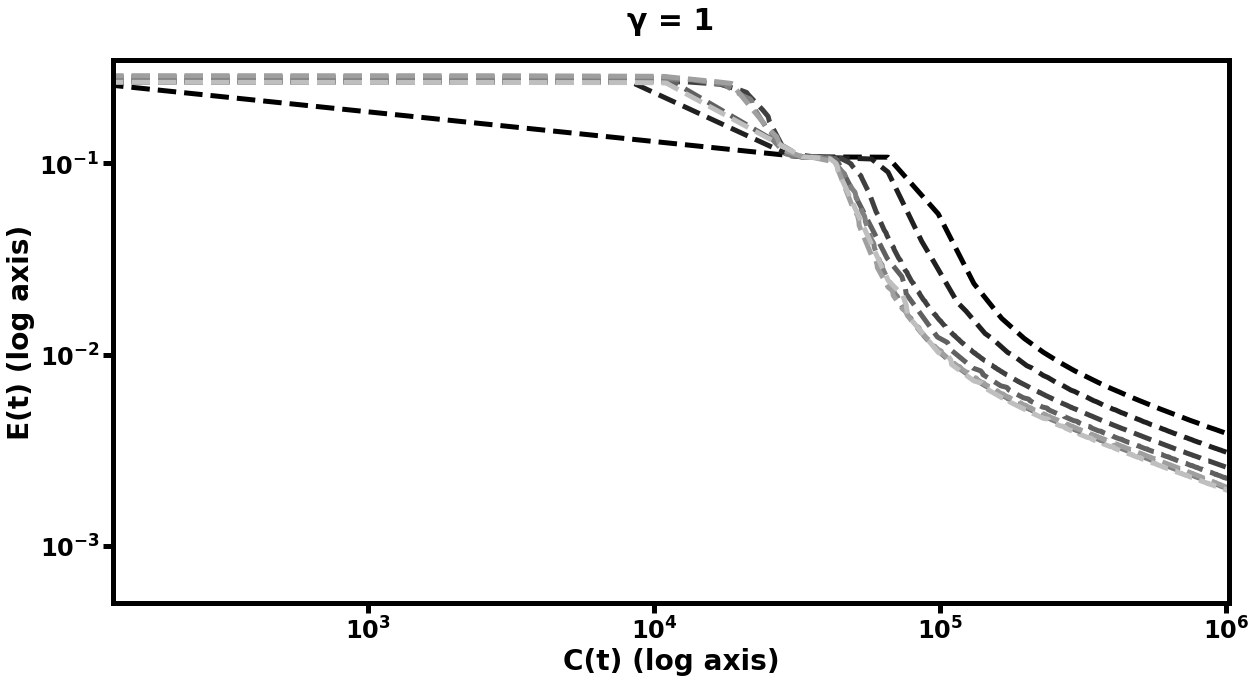
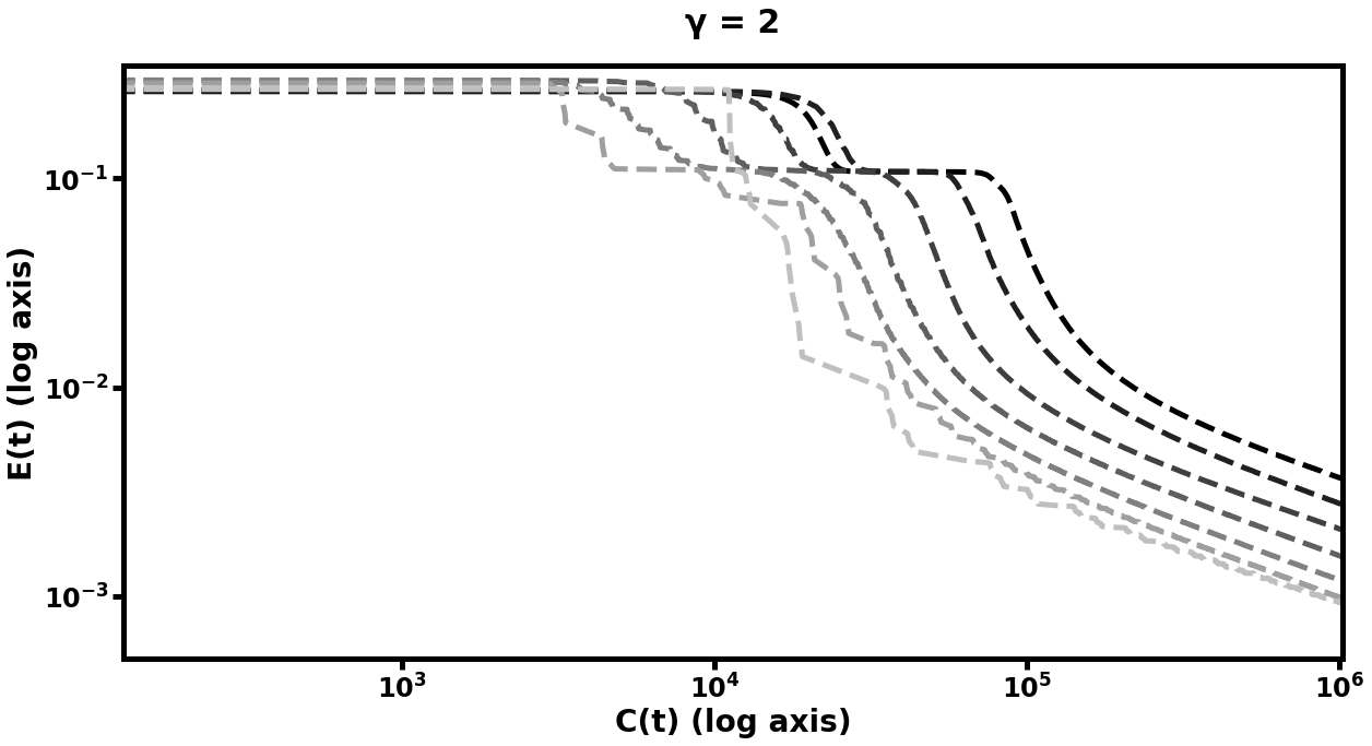
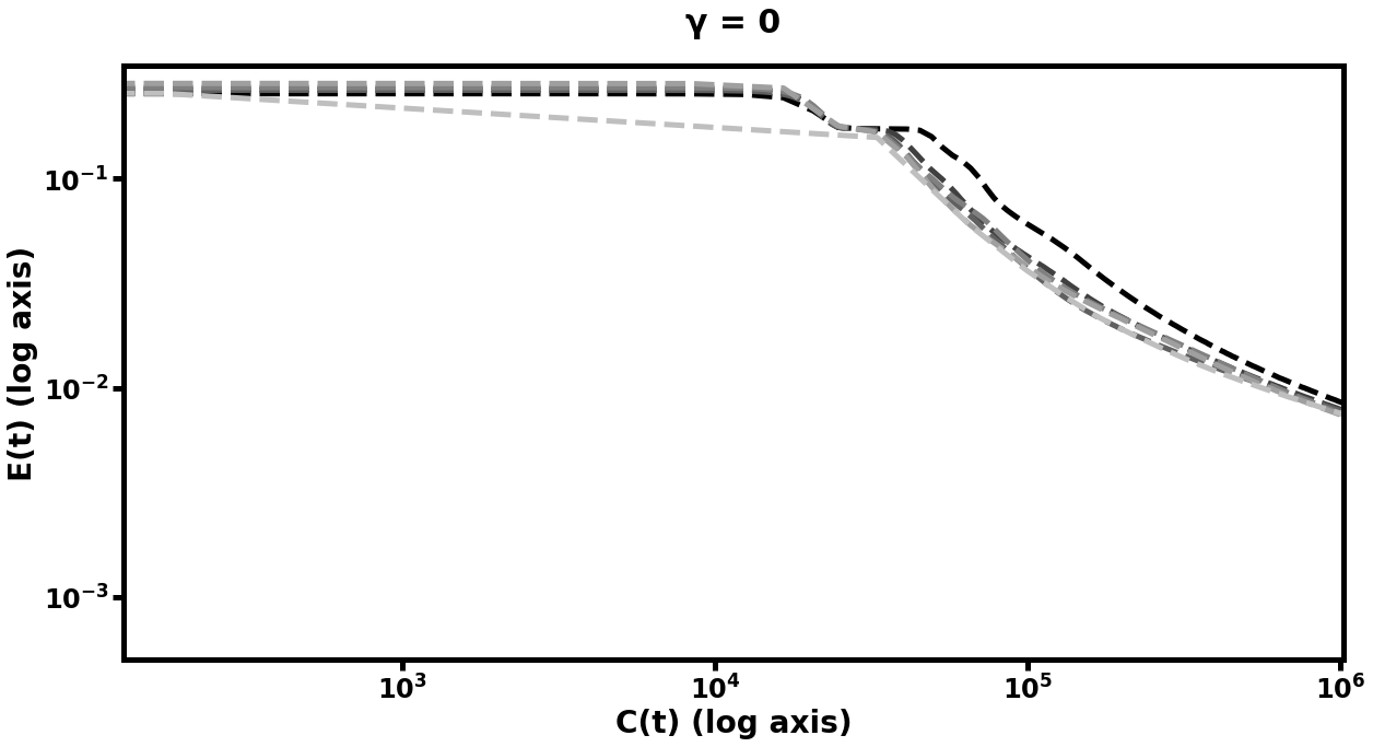
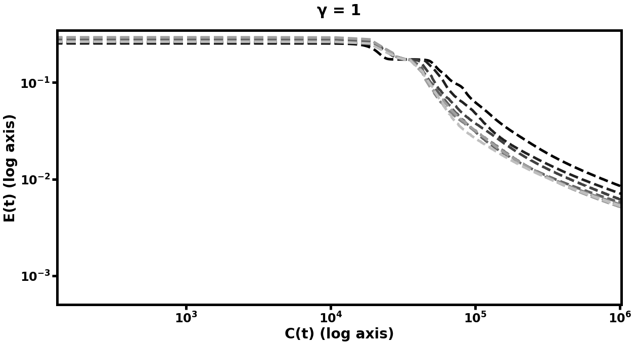
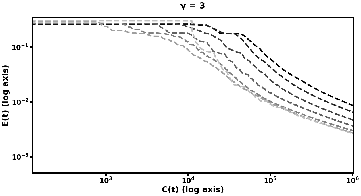
The results of this experiment are plotted in Figure [fig:autofig] and summarized in Table [tbl:oneobj]. We perform multiple runs of the entire training procedure with differing values of $k$ (the number of smoothing steps), $\gamma$ (the multigrid cycle parameter), and $L$ (depth of hierarchy). Notably, nearly all multigrid schedules demonstrate performance gains over the default network (i.e. the network which trains only at the $l=0$ scale), with more improvement for higher values of $k$ , $L$ , and $\gamma$ . The hierarchy which learned most rapidly was the deepest model $(L=6)$ with $k = 4$ and $\gamma = 3$ . Those multigrid models which did not improve over the default network were only slightly more computationally expensive per unit of accuracy than their default counterparts, and the multigrid models which did improve, improved significantly.

$Log-log plots of accuracy E(t) as a function of training cost C(t) attained by a variety of hierarchical neural networks training on a simple machine vision task, demonstrating that deeper hierarchies with more mutligrid behavior learn more rapidly. Plots are ordered from top to bottom in increasing depth of recursion parameter \gamma; left plots are the single-object experiments and right plots are the double-object experiments. Within each plot, different curves represent different values of the depth of hierarchy, from L=6 (lightest) to L=0 (darkest). Each line is the best run for that pair (L, \gamma) over all choices of k (number of smoothing steps at each level) in \{1,2,4,8,16,32,64,128\}.$
$Log-log plots of accuracy E(t) as a function of training cost C(t) attained by a variety of hierarchical neural networks training on a simple machine vision task, demonstrating that deeper hierarchies with more mutligrid behavior learn more rapidly. Plots are ordered from top to bottom in increasing depth of recursion parameter \gamma; left plots are the single-object experiments and right plots are the double-object experiments. Within each plot, different curves represent different values of the depth of hierarchy, from L=6 (lightest) to L=0 (darkest). Each line is the best run for that pair (L, \gamma) over all choices of k (number of smoothing steps at each level) in \{1,2,4,8,16,32,64,128\}.$
$Log-log plots of accuracy E(t) as a function of training cost C(t) attained by a variety of hierarchical neural networks training on a simple machine vision task, demonstrating that deeper hierarchies with more mutligrid behavior learn more rapidly. Plots are ordered from top to bottom in increasing depth of recursion parameter \gamma; left plots are the single-object experiments and right plots are the double-object experiments. Within each plot, different curves represent different values of the depth of hierarchy, from L=6 (lightest) to L=0 (darkest). Each line is the best run for that pair (L, \gamma) over all choices of k (number of smoothing steps at each level) in \{1,2,4,8,16,32,64,128\}.$
$Log-log plots of accuracy E(t) as a function of training cost C(t) attained by a variety of hierarchical neural networks training on a simple machine vision task, demonstrating that deeper hierarchies with more mutligrid behavior learn more rapidly. Plots are ordered from top to bottom in increasing depth of recursion parameter \gamma; left plots are the single-object experiments and right plots are the double-object experiments. Within each plot, different curves represent different values of the depth of hierarchy, from L=6 (lightest) to L=0 (darkest). Each line is the best run for that pair (L, \gamma) over all choices of k (number of smoothing steps at each level) in \{1,2,4,8,16,32,64,128\}.$

Double-Object Autoencoder

We repeat the above experiment with a slightly more difficult machine vision task - the network must learn to de-noise an image with two (non-overlapping) ‘objects’ in the visual field. We use the same network structure and training procedure, and note that we see again (plotted in Figure [fig:autofig] and summarized in Table [tbl:twoobj]) that the hierarchical model is more efficient, reaching lower error in the same amount of computational cost $C(t)$ . The multigrid neural networks again typically learn much more rapidly than the non-multigrid models.

MNIST

To supplement the above synthetic experiments with one using real-world data, we perform the same experiment with an autoencoder for the MNIST handwritten digit dataset (LeCun et al. 1998; LeCun, Cortes, and Burges 2010). In this case, rather than the usual MNIST classification task, we use an autoencoder to map the MNIST images into a lower-dimensional $(d=128)$ space with good reconstruction. We use the same network structure as in the 1D vision example; also as in that example, each network in the hierarchy is constructed of fully connected layers with bias terms and sigmoid activation, and smoothing steps are performed with RMSProp (Hinton, Srivastava, and Swersky, n.d.) with learning rate 0.0005. The only difference is that in this example we do not add noise to the input images, since the dataset is larger by two orders of magnitude.

In this experiment, we see (in Figure [fig:mnistfig] and Table [tbl:mnist]) similar improvement in efficiency. Table [tbl:mnist] summarizes these results: the best multilevel models learned more rapidly and achieved lower error than their single-level counterparts, whereas the worst multilevel models performed on par with the default model. Because the MNIST data is comprised of 2D images, we tried using $P$ matrices which were the optima of prolongation problems between grids of the appropriate sizes, in addition to the same 1D $P$ used in the prior two experiments. The difference in performance between these two choices of underlying structure for the prolongation maps can be seen in Figure [fig:mnistfig]. With either approach, we see similar results to the synthetic data experiment, in that more training steps at the coarser layers results in improved learning performance of the finer networks in the hierarchy. However, the matrices optimized for 2D prolongation perform marginally better than their 1D cousins, - in particular, the multigrid hierarchy with 2D prolongations took 60% of the computational cost to reduce its error to $\frac{1}{10}$ of its original value, as compared to the 1D version. We explore the effect of varying the strategy used to pick $P$ in Subsection 6.5.3.

Experiments of Choice of $P$

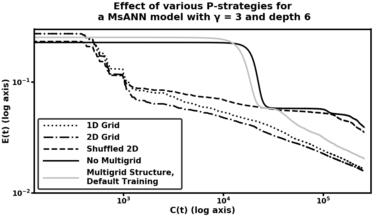
To further explore the role of the structure of $P$ in these machine learning models, we compare the performance of several MsANN models with $P$ generated according to various strategies. Our initial experiment on the MNIST dataset used the exact same hierarchical network structure and prolongation/restriction operators as the example with 1D data, and yielded marginal computational benefit. We were thus motivated to try this learning task with prolongations which are designed for for 2D grid-based model architectures, as well as trying unstructured (random orthogonal) matrices as a baseline. More precisely, our 1D experiments used $P$ matrices resembling those in column 3 of the “Cycle Graphs" section of Figure [fig:pspeciesfig]. We instead, for the MNIST task, used $P$ matrices like those in column $6$ of the “Grid Graphs” section of the same figure. In Figure [fig:pcomp_mnist], we illustrate the difference in these choices for the MNIST training task, with the same choice of multigrid training parameters: $(L = 6, \gamma = 3, k = 1)$ . We compare the following strategies for generating $P$ :

[misc:plist_elem_0] As local optima of a prolongation problem between 1D grids, with periodic boundary conditions;
[misc:plist_elem] As local optima of a prolongation problem between 2D grids, with periodic boundary conditions;
[misc:plist_elem_2] As in [misc:plist_elem], but shuffled along the first index of the array.

Strategy [misc:plist_elem_2] was chosen to provide the same degree of connectivity between each coarse variable and its related fine variables as strategy [misc:plist_elem], but in random order i.e. connected in a way which is unrelated to the 2D correlation between neighboring pixels. We see in Figure [fig:pcomp_mnist] that the two strategies utilizing local optima outperform both the randomized strategy and default training (training only the finest scale). Furthermore, strategy [misc:plist_elem] outperforms strategy [misc:plist_elem_0], although the latter eventually catches up at the end of training, when coarse-scale weight training has diminishing marginal returns. The random strategy is initially on par with the two optimized ones (we speculate that this is due to the ability to affect many fine-scale variables at once, even in random order, which may make the gradient direction easier to travel), but eventually falls behind, at times being less efficient than default training. We leave for further work the question of whether there are choices of prolongation problem which are even more efficient for this machine learning task. We also compare all of the preceeding models to a model which has the same structure as a MsANN model (a hierarchy of coarsened variables with $\text{Pro}$ and $\text{Res}$ operators between them), but which was trained by training all variables in the model simultaneously. This model performs on par with the default model, illustrating the need for the multilevel training schedule dictated by the choice of $\gamma$ .

Comparison of several choices of \text{Pro} and \text{Res} operators for a Multiscale Neural Network training experiment, on MNIST data. Two choices for P which are local optima of prolongation problems demonstrate more efficient training than default, while two strategies perform worse: multigrid training with random P matrices, and training all varibles in the hierarchy simultaneously. — Comparison of several choices of $\text{Pro}$ and $\text{Res}$ operators for a Multiscale Neural Network training experiment, on MNIST data. Two choices for $P$ which are local optima of prolongation problems demonstrate more efficient training than default, while two strategies perform worse: multigrid training with random $P$ matrices, and training all varibles in the hierarchy simultaneously.

[fig:pcomp_mnist]

Summary

We see uniform improvement (as the parameters $L$ and $\gamma$ are increased) in the rate of neural network learning when models are stacked in the type of multiscale hierarchy we define in equations [eqn:weightpro] and [eqn:biaspro], despite the diversity of machine learning tasks we examine. Furthermore, this improvement is marked: the hierarchical models both learn more rapidly than training without multigrid and have final error lower than the default model. In many of our test cases, the hierarchical models reached the same level of MSE as the default in more than an order of magnitude fewer training examples, and continued to improve, surpassing the final level of error reached by the default network. Even in the worst case, our hierarchical model structure performed on par with neural networks which did not incorporate our weight prolongation and restriction operators. We leave the question of finding optimal $(L, \gamma, k)$ for future work - see Section 6.6 for further discussion. Finally, we note that the model(s) in the experiments presented in section 6.5.1 were essentially the same MsANN models (same set of $L, \gamma, k$ and same set of $P$ matrices), and showed similar performance gains on two different machine vision problems, indicating that it may be possible to develop general MsANN model-creation procedures that are applicable to a variety of problems (rather than needing to be hand-tuned).

Conclusion and Future Work

We have introduced a novel method for multiscale modeling, which relies on a novel prolongation and restriction operator to move between models in a hierarchy. These prolongation and restriction operators are the optima of an objective function we introduce which is a natural distance metric on graphs and graph lineages. We prove several important properties of this objective function, including an upper bound which allows us to decouple a difficult optimization into two smaller optimization problems under certain circumstances.

Additionally, we demonstrate an algorithm which makes use of such $P$ and $R$ operators to simultaneously train models in a hierarchy of neural networks (specifically, autoencoder neural networks). This Multiscale Artificial Neural Network (MsANN) approach statistically outperforms training only at the finest scale, achieving lower error than the default model and also reaching the default model’s best performance in an order of magnitude fewer training examples. While in our experiments we saw uniform improvement as the parameters $\gamma$ , $k$ , and $L$ were increased (meaning that the hierarchy is deeper, and the model spends more relative time training at the coarser scales), this may not always be the case, and we leave the question of finding optimal settings of these parameters for future work.

Promising directions for future work also include investigating the properties of the distance metric on graphs, and the use of those properties in graph lineage, as well as modifying the MsANN algorithm to perform the same type of hierarchical learning on more complicated ANN models, such as Convolutional Neural Networks (CNNs), as well as non-autoencoding tasks, for example classification.