Numerical Properties of GDD

Graph Lineages

In this section we introduce several specific graph lineages for which we will compute various intra- and inter-lineage distances. Three of these are well-known lineages of graphs, and the fourth is defined in terms of a product of complete graphs:

Path Graphs ($\text{Pa}_n$): 1D grid graphs of length $n$, with aperiodic boundary conditions.

Cycle Graphs ($\text{Cy}_n$): 1D grid graphs of length $n$, with periodic boundary conditions.

Square Grid Graphs ($\text{Sq}_n$): 2D grid graphs of dimensions $n$, with aperiodic boundary conditions. $\text{Sq}_n = \text{Pa}_n \Box \text{Pa}_n$

“Multi-Barbell” Graphs ($\text{Ba}_n$): Constructed as $\text{Cy}_n \Box K_n$, where $K_n$ is the complete graph on $n$ vertices.

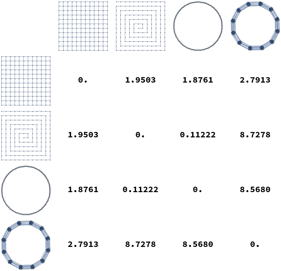
These familes are all illustrated in Figure [fig:graph_families].

2D Grids

Paths

Cycles

k-Barbell graphs

[fig:graph_families]

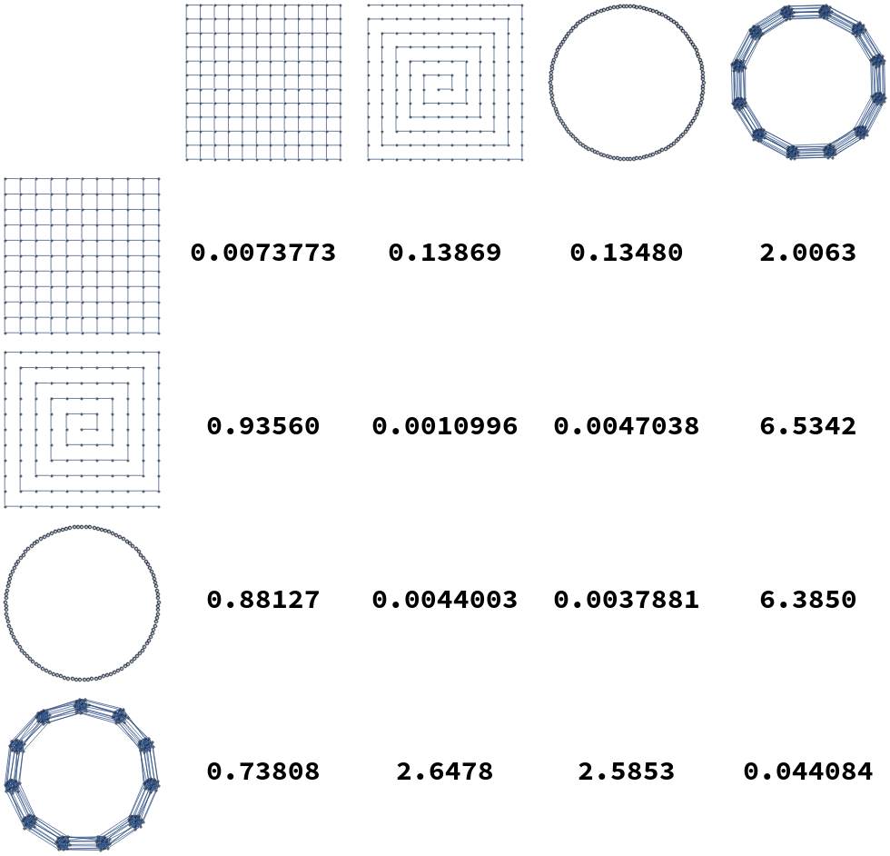
Additionally, some examples distances between elements of these graph lineages are illustrated in Figure [fig:gdist_plots]. In these tables we see that in general intra-lineage distances are small, and inter-lineage distances are large.

[fig:gdist_plots]

Numerical Optimization Methods

We briefly discuss here the other numerical methods we have used to calculate $\tilde{D}^2$ and $D^2$. In general we have found these methods inferior to the algoithm presented in Chapter 4, but we present them here for completeness.

Nelder-Mead in Mathematica For very small graph pairs ($n_1 \times n_2 \leq 100$) we are able to find optimal $P, \alpha, t$ using constrained optimization in Mathematica 11.3 (Inc., n.d.) using NMinimize, which uses Nelder-Mead as its backend by default. The size limitation made this approach unusable for any real experiments.

Orthogonally Constrained Opt. We also tried a variety of codes specialized for numeric optimization subject to orthogonality constraints. These included (1) the python package PyManopt (Townsend, Koep, and Weichwald 2016), a code designed for manifold-constrained optimization; (2) gradient descent in Tensorflow using the penalty function $g(P) = c {\left| \left| P^T P - I \right| \right|}_F$ (with $c \ll 1$ a small positive constant weight) to maintain orthogonality, as well as (3) an implementation of the Cayley reparametrization method from (Wen and Yin 2013) (written by the authors of that same paper). In our experience, these codes were slower, with poorer scaling with problem size, than combinatorial optimization over subpermutation matrices, and did not produce improved results on our optimization problem.

Black-Box Optimization Over $\alpha$.

We compare in more detail two methods of joint optimization over $\alpha$ and $P$ when $P$ is constrained to be a subpermutation matrix in the diagonal basis for $L(G_1)$ and $L(G_2)$. Specifically, we compare our approach given in Algorithm [alg:linear_alg] to univariate optimization over $\alpha$, where each function evaluation consists of full optimization over $P$. Figure [fig:alg_timing] shows the results of this experiment. We randomly sample pairs of graphs as follows:

1. $n_1$ is drawn uniformly from $[ 5, 120]$.

2. $n_2$ is drawn uniformly from $[n_1, n_1 + 60 ]$.

3. $G_1$ and $G_2$ are generated by adding edges according to a Bernoulli distribution with probability $p$. We ran 60 trials for each $p$ in { .125, .25, .375, .5, .625, .75, .875 }.

We compute the linear version of distance for each pair. Because our algorithm finds all of the local minima as a function of alpha, we compute the cost of the golden section approach as the summed cost of multiple golden section searches in alpha: one GS search starting from the initial bracket $[0.618 \alpha^*, 1.618 \alpha^*]$ for each local minimum $\alpha^*$ found by our algorithm. We see that our algorithm is always faster by at least a factor of 10, and occasionally faster by as much as a factor of $10^3$. This can be attributed to the fact that the golden section search is unaware of the structure of the linear assignment problem: it must solve a full $n_2 \times n_2$ linear assignment problem for each value of $\alpha$ it explores. In contrast, our algorithm is able to use information from prior calls to the LAP solver, and therefore solves a series of LAP problems whose sizes are monotonically nonincreasing.

[fig:alg_timing]

Triangle Inequality violation of $D$ (Exponential Distance) and $\tilde{D}$ (Linear Distance)

As stated in Section 2.3, our full graph dissimilarity measure does not necessarily obey the triangle inequality. In this section we systematically explore conditions under which the triangle inequality is satisfied or not satisfied. We generate triplets $G_1, G_2, G_3$ of random graphs of sizes $n_i$ for $n_1 \in [5, 30]$, $n_2 \in [n_1, n_1 + 30]$, and $n_3 \in [n_2, n_2 + 30]$ by drawing edges from the Bernoulli distribution with probability $p$ (we perform 4500 trials for each $p$ value in [.125, .25, .375, .5, .625, .75, .875]). We compute the distance $\tilde{D}(G_i, G_k)$ (for $(i,k) \in \{ (1,3), (1,2), (2,3) \}$). The results may be seen in Figure [fig:triangle_ineq_histogram]. In this figure we plot a histogram of the “discrepancy score” $$\begin{aligned} \text{Disc}(G_1, G_2, G_3) = \tilde{D}(G_1, G_3)/(\tilde{D}(G_1, G_2) + \tilde{D}(G_2, G_3)),\end{aligned}$$ which measures the degree to which a triplet of graphs violates the triangle inequality (i.e. falls outside of the unit interval [0,1]), for approximately $3 \times 10^4$ such triplets. It is clear that, especially for the linear definition of the distance, the triangle inequality is not always satisfied. However, we also observe that (for graphs of these sizes) the discrepancy score is bounded: no triple violates the triangle inequality by more than a factor of approximately 1.8. This is shown by the histogram of discrepancies in Figure [fig:triangle_ineq_histogram]. Additionally, the triangle inequality is satisfied in 28184 (95.2%) of cases.

We see similar but even stronger results when we run the same experiment with $D^2$ instead of $\tilde{D}^2$; these may also be seen in Figure [fig:triangle_ineq_histogram]. We calculated the discrepancy score analogously, but with $D$ substituted for $\tilde{D}$. We see similarly that the degree of violation is bounded. In this case, no triple violated the triangle inequality by a factor of more than 5, and in this case the triangle inequality was satisfied in 99.8% of the triples. More work is needed to examine this trend; in particular, it would be interesting to examine whether other models of graph generation also satisfy the triangle inequality up to this constant. In both of these cases, the triangle inequality violations may be a result of our optimization procedure finding local minima/maxima for one or more of the three distances computed. We also repeat the above procedure for the same triplets of graphs, but with distances computed not in order of increasing vertex size: calculating $\text{Disc}(G_2, G_1, G_3)$ and $\text{Disc}(G_3, G_2, G_1)$. All of these results are plotted in Figure [fig:triangle_ineq_histogram].

[fig:triangle_ineq_histogram]

Intra- and Inter-Lineage Distances

We compute pairwise distances for sequences of graphs in the graph lineages displayed in Figure [fig:graph_families]. For each pair of graph families (Square Grids, Paths, Cycles, and Multi-Barbells), we compute the distance from the $i$th member of one lineage to the $(i+1)$-st member of each other lineage, and take the average of the resulting distances from $i=1$ to $i=12$. These distances are listed in Table [tab:dist_table]. As expected, average distances within a lineage are smaller than the distances from one lineage to another.

[tab:dist_table]

We note here that the idea of computing intra- and inter- lineage distances is similar to recent work (Hartle et al. 2020) computing distances between graph ensembles: certain classes of similarly-generated random graphs. Graph diffusion distance has been previously shown (in (Hartle et al. 2020)) to capture key structural information about graphs; for example, GDD is known to be sensitive to certain critical transitions in ensembles of random graphs as the random parameters are varied. This is also true for our time dilated version of GDD. More formally: let $G_p$ and $G_p^{'}$ represent random graphs on $n$ vertices, drawn from the Erdős-Renyi distribution with edge probability $p$. Then $D(G_p, G_p^{'})$ has a local maximum at $p=\frac{1}{n}$, representing the transition between disconnected and connected graphs. This is true for our distance as well as the original version due to Hammond.

Graph Limits

Here, we provide preliminary evidence that graph distance measures of this type may be used in the definition of a graph limit - a graphlike object which is the limit of an infinite sequence of graphs. This idea has been previously explored, most famously by Lovász (Lovász 2012), whose definition of a graph limit (called a graphon) is as follows: Recall the definition of graph cut-distance $D_{\text{cut}}(G, H)$ from Equation [defn:cut_dist], namely: the cut distance is the maximum discrepancy in sizes of edge-cuts, taken over all possible subsets of vertices, between two graphs on the same vertex-set. A graphon is then an equivalence class of Cauchy sequences of graphs1, under the equivalence relation that two sequences $G_1, G_2, \ldots$ and $H_1, H_2, \ldots$ are equivalent if $D_{\text{cut}}(G_i, H_i)$ approaches 0 as $n \rightarrow \infty$.

We propose a similar definition of graph limits, but with our diffusion distance substituted as the distance measure used in the definition of a Cauchy sequence of graphs. Hammond et. al. argue in (Hammond, Gur, and Johnson 2013) why their variant of diffusion distance may be a more descriptive distance measure than cut-distance. More specifically, they show that on some classes of graphs, some edge deletions ‘matter’ much more than others: removal of a single edge changes the diffusive properties of the graph significantly. However, the graph-cut distance between the new and old graphs is the same, regardless of which edge has been removed, while the diffusion distance captures this nuance. For graph limits, however, our generalization to unequal-sized graphs via $P$ is of course essential. Furthermore, previous work (Borgs et al. 2019) on sparse graph limits has shown that in the framework of Lovász all sequences of sparse graphs converge (in the infinite-size limit) to the zero graphon. Graph convergence results specific to sparse graphs include the Benjamini-Schramm framework (Benjamini and Schramm 2001), in which graph sequences are compared using the distributional limits of subgraph frequencies. These two graph comparison methods both have the characteristic that the “limit object” of a sequence of graphs is rigorously defined. It is unclear that density functions on the unit square are the best choice of limit objects for graphs; while graphons have many nice properties as detailed by Lovász, other underlying limit objects may be a more natural choice for sparse graphs. In this section we attempt to show empirically that such a limit object of graph sequences under GDD may exist, and therefore merit further investigation.

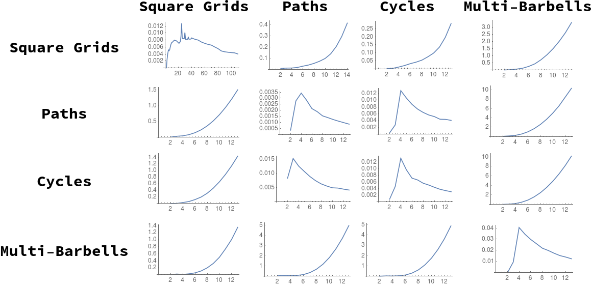
We examine several sequences of graphs of increasing size for the required Cauchy behavior (in terms of our distance measure) to justify this variant definition of a “graph limit”. For each of the graph sequences defined in Section 5.1, we examine the distance between successive members of the sequence, plotting $D^2(G_n, H_{n+1})$ for each choice of $G$ and $H$. These sequences of distances are plotted in Figure [fig:g_limits].

In this figure, we see that generally distance diverges between different graph lineages, and converges for successive members of the same lineage, as $n \rightarrow \infty$. We note the exceptions to this trend:

1. The distances between $n$-paths and $n+1$-cycles appear to be converging; this is intuitive, as we would expect that difference between the two spectra due to distortion from the ends of the path graph would decrease in effect as $n \rightarrow \infty$.

2. We also show analytically, under similar assumtions, that the distance between successive path graphs also shrinks to zero (Theorem [thm:pa_lim_lem]).

We do not show that all similarly-constructed graph sequences display this Cauchy-like behavior. We hope to address this deeper question, as well as a more formal exploration of the limit object, with one or more modified versions of the objective function (see Section 3.8.1).

Limit of Path Graph Distances

In this section, we demonstrate analytically that the sequence of path graphs of increasing size is Cauchy in the sense described by the previous section. In the following theorem (Theorem [thm:pa_lim_lem]), we assume that the optimal value of $t$ approaches some value $\tilde{t}$ as $n \rightarrow \infty$. We have not proven this to be the case, but have observed this behavior for both square grids and path graphs (see Figure [fig:path_lim] for an example of this behavior). Lemmas [lem:path_eigen_limit] and [thm:pa_lim_lem] show a related result for path graphs; we note that the spectrum of the Laplacian (as we define it in this paper) of a path graph of size $n$ is given by $$\begin{aligned} \lambda_k = -2 + 2 \cos{\frac{k \pi}{n - 1}} \quad \quad k \in \{0 ... n-1\}. \nonumber \end{aligned}$$

[lem:path_eigen_limit] For any finite $k, t$, we have $$\begin{aligned} \lim_{n \rightarrow \infty} n {\left( e^{t(-2 + 2 \cos(\frac{\pi k}{n}))} - e^{t(-2 + 2 \cos(\frac{\pi k}{n+1}))} \right)}^2 = 0 \nonumber\end{aligned}$$

Clearly for finite $k,t$ $$\begin{aligned} \lim_{n \rightarrow \infty} {\left( e^{t(-2 + 2 \cos(\frac{\pi k}{n}))} - e^{t(-2 + 2 \cos(\frac{\pi k}{n+1}))} \right)} = 0 \nonumber\end{aligned}$$ Then, $$\begin{aligned} &\lim_{n \rightarrow \infty} n {\left( e^{-2 + 2 \cos(\frac{\pi k}{n})} - e^{-2 + 2 \cos(\frac{\pi k}{n+1})} \right)} \nonumber \\ &\quad \quad \quad = \lim_{n \rightarrow \infty} \frac{ {\left( e^{-2 + 2 \cos(\frac{\pi k}{n})} - e^{-2 + 2 \cos(\frac{\pi k}{n+1})} \right)}}{\frac{1}{n}} \nonumber\end{aligned}$$ Evaluating this expression requires applying L’Hôpital’s rule. Hence, we have: $$\begin{aligned} &\lim_{n \rightarrow \infty} \frac{ {\left( e^{-2 + 2 \cos(\frac{\pi k}{n})} - e^{-2 + 2 \cos(\frac{\pi k}{n+1})} \right)}}{\frac{1}{n}} \nonumber \\ &\quad \quad = \lim_{n \rightarrow \infty} \frac{ 2 \pi k t \left(\frac{\sin \left(\frac{\pi k}{n}\right) e^{2 t \left(\cos \left(\frac{\pi k}{n}\right)-1\right)}}{n^2}-\frac{\sin \left(\frac{\pi k}{n+1}\right) e^{2 t \left(\cos \left(\frac{\pi k}{n+1}\right)-1\right)}}{(n+1)^2}\right) }{\frac{-1}{n^2}} \nonumber \\ &\quad \quad = 2 \pi k t \lim_{n \rightarrow \infty} \left(\frac{n^2 \sin \left(\frac{\pi k}{n+1}\right) e^{2 t \left(\cos \left(\frac{\pi k}{n+1}\right)-1\right)}}{(n+1)^2}-\sin \left(\frac{\pi k}{n}\right) e^{2 t \left(\cos \left(\frac{\pi k}{n}\right)-1\right)}\right). \nonumber \end{aligned}$$ Since both of the limits $$\begin{aligned} \lim_{n \rightarrow \infty} \left(\frac{n^2 \sin \left(\frac{\pi k}{n+1}\right) e^{2 t \left(\cos \left(\frac{\pi k}{n+1}\right)-1\right)}}{(n+1)^2} \right) \nonumber \\ \intertext{and} \lim_{n \rightarrow \infty} \left(-\sin \left(\frac{\pi k}{n}\right) e^{2 t \left(\cos \left(\frac{\pi k}{n}\right)-1\right)}\right) \nonumber \end{aligned}$$ exist (and are 0), $$\begin{aligned} & 2 \pi k t \lim_{n \rightarrow \infty} \left(\frac{n^2 \sin \left(\frac{\pi k}{n+1}\right) e^{2 t \left(\cos \left(\frac{\pi k}{n+1}\right)-1\right)}}{(n+1)^2}-\sin \left(\frac{\pi k}{n}\right) e^{2 t \left(\cos \left(\frac{\pi k}{n}\right)-1\right)}\right) =0 \nonumber \intertext{and therefore} & \lim_{n \rightarrow \infty} n {\left( e^{t(-2 + 2 \cos(\frac{\pi k}{n}))} - e^{t(-2 + 2 \cos(\frac{\pi k}{n+1}))} \right)}^2 = 0 \nonumber\end{aligned}$$

[thm:pa_lim_lem] If $\lim_{n \rightarrow \infty} \arg \sup_t D^2\left( \left. \text{\emph{Pa}}_n, \text{\emph{Pa}}_{n+1} \right| t \right)$ exists, then: $$\begin{aligned} \lim_{n \rightarrow \infty} D^2 \left( \text{Pa}_n, \text{Pa}_{n+1} \right) = 0. \nonumber\end{aligned}$$

Assume that $\lim_{n \rightarrow \infty} \arg \sup_t D^2\left( \left. \text{Pa}_n, \text{Pa}_{n+1} \right| t \right) = \tilde{t}$. Then, we must have $$\begin{aligned} \lim_{n \rightarrow \infty} D^2 \left( \text{Pa}_n, \text{Pa}_{n+1} \right) &\leq \lim_{n \rightarrow \infty} D^2 \left( \left. \text{Pa}_n, \text{Pa}_{n+1} \right| \tilde{t} \right) \nonumber\end{aligned}$$ Hence, it remains only to prove that $$\begin{aligned} \lim_{n \rightarrow \infty} D^2 \left( \left. \text{Pa}_n, \text{Pa}_{n+1} \right| t \right) = 0 \nonumber\end{aligned}$$ for any finite $t$ (which will then include $\tilde{t}$). First, for any particular $( n + 1) \times n$ subpermutation matrix $S$, note that

$$\begin{aligned} D^2 \left( \left. \text{Pa}_n, \text{Pa}_{n+1} \right| t \right) &= \inf_{\alpha > 0} \inf_{P | \mathcal{C}(P)} D^2 \left( \left. \text{Pa}_n, \text{Pa}_{n+1} \right| t, P, \alpha \right) \nonumber \\ &\leq D^2 \left( \left. \text{Pa}_n, \text{Pa}_{n+1} \right| t, \alpha=1 , U_{n+1}^T S U_n\right) \nonumber\end{aligned}$$ Here, $U_n$ and $U_{n+1}$ are the matrices which diagonalize $L(\text{Pa}_n)$ and $L(\text{Pa}_{n+1})$ respectively (note also that a diagonalizer of a matrix $L$ also diagonalizes $e^{L}$). If at each $n$ we select $S$ to be the subpermutation $S = \left[ \begin{array}{c} I \\ 0 \end{array}\right]$, then (using the same argument as in Theorem [thm:LAP_bound]) the objective function simplifies to: $$\begin{aligned} & D^2\left(\text{Pa}_n, \text{Pa}_{n+1} \right| t, P = U_{n+1}^T S U_n, \alpha=1) \nonumber \\ &\quad = {\left| \left| S e^{c \Lambda_{\text{Pa}_n}} - e^{c \Lambda_{\text{Pa}_{n+1}}} S \right| \right|}_F^2 \nonumber \\ &\quad = \sum_{k=0}^{n-1} {\left( e^{c(-2 + 2 \cos(\frac{\pi k}{n}))} - e^{c(-2 + 2 \cos(\frac{\pi k}{n+1}))} \right)}^2 \nonumber \\ &\quad \leq \max_{0 \leq k \leq n-1} n {\left( e^{c(-2 + 2 \cos(\frac{\pi k}{n}))} - e^{c(-2 + 2 \cos(\frac{\pi k}{n+1}))} \right)}^2 \nonumber\end{aligned}$$ By Lemma [lem:path_eigen_limit], for any finite $k, t$, we have $$\begin{aligned} \lim_{n \rightarrow \infty} n {\left( e^{t(-2 + 2 \cos(\frac{\pi k}{n}))} - e^{t(-2 + 2 \cos(\frac{\pi k}{n+1}))} \right)}^2 = 0 \nonumber\end{aligned}$$ So for any $\epsilon > 0$, $\exists N$ such that when $n \geq N$, for any $c, k$, $$\begin{aligned} n {\left( e^{c(-2 + 2 \cos(\frac{\pi k}{n}))} - e^{c(-2 + 2 \cos(\frac{\pi k}{n+1}))} \right)}^2 < \epsilon \nonumber\end{aligned}$$ But then $$\begin{aligned} \sum_{k=0}^{n-1} {\left( e^{c(-2 + 2 \cos(\frac{\pi k}{n}))} - e^{c(-2 + 2 \cos(\frac{\pi k}{n+1}))} \right)}^2 < \epsilon \nonumber\end{aligned}$$ as required. Thus, the Cauchy condition is satisfied for the lineage of path graphs $\text{Pa}_n$

[fig:path_lim]

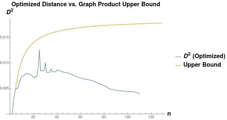
Given a graph lineage which consists of levelwise box products between two lineages, it seems natural to use our upper bound on successive distances between graph box products to prove convergence of the sequence of products. As an example, the lineage consisting of square grids is the levelwise box product of the lineage of path graphs with itself. However, in this we see that this bound may not be very tight. Applying Equation [eqn:graph_product_special_case] from Theorem [thm:sq_grid_lim_lem], we have (for any $t_c, \alpha_c$): $$\begin{aligned} D \left( \left. \text{Sq}_n, \text{Sq}_{n+1} \right. \right) &\leq D \left( \left. \text{Sq}_n, \text{Sq}_{n+1} \right| t_c, \alpha_c \right) \nonumber \\ &\leq D \left( \text{Pa}_{n+1}, \text{Pa}_{n+1} \left. \right| t_c, \alpha_c \right) \left( {\left| \left| e^{\frac{t_c}{a_c} L(\text{Pa}_n)} \right| \right|}_F \right. \nonumber \\ & \quad \quad \quad \quad + \left. {\left| \left| e^{t_c a_c L(\text{Pa}_{n+1})} \right| \right|}_F \right) \nonumber \end{aligned}$$ As we can see in Figure [fig:sq_dist_vs_bound], the right side of this inequality seems to be tending to a nonzero value as $n \rightarrow \infty$, whereas the actual distance (calculated by our optimization procedure) appears to be tending to zero.

[fig:sq_dist_vs_bound]

[fig:g_limits]